Chapter 9 Two-sample tests
9.1 Motivation
Question: Is there some form of dependence between two variables \(X\) and \(Y\)? Does the knowledge about the realization of \(X\) also convey information about \(Y\)?
Often: One of the variables (\(Y\)) is the dependent variable, the other (\(X\)) is independent or explanatory. If both variables enter equally, the roles may also be interchangeable.
Exploratory: Bivariate exploratory analysis (see Chapter 4.2).
Inference: Various tests for the hypothesis pair
- \(H_0:\) Independence of \(X\) and \(Y\).
- \(H_1:\) Some form of dependence between \(X\) and \(Y\).
Testing procedures differ depending on the scale level of the two variables but also with respect to the type of putative form of dependence under the alternative.
| Dep. vs. expl. | Quantitative | Qualitative |
|---|---|---|
| Quantitative | Correlation tests (Pearson, Spearman, …) |
2- and k-sample tests (t-test, analysis of variance, Wilcoxon-Mann-Whitney, …) |
| Qualitative | Logistic regression (bi-, multinomial, …) |
\(\chi^2\)-test, Fisher’s exact test, … |
Initially: Consider the 2-sample problem, i.e., a dependent quantitative variable \(Y\) and a binary explanatory variable \(X\). The binary variable \(X\) splits the variable \(Y\) into two subsamples.
Jargon: 2-sample testing is also known as A/B testing, especially for randomized experiments with two experimental conditions.
Especially: Popular jargon in e-commerce. Under varying setups of a web page, assess:
- Revenue generated.
- Click-through rate.
- Number of purchases.
- Transactions per user.
9.2 Comparison of distributions
Task: Assess several distributions for differences.
- \(H_0:\) All samples come from the same distribution.
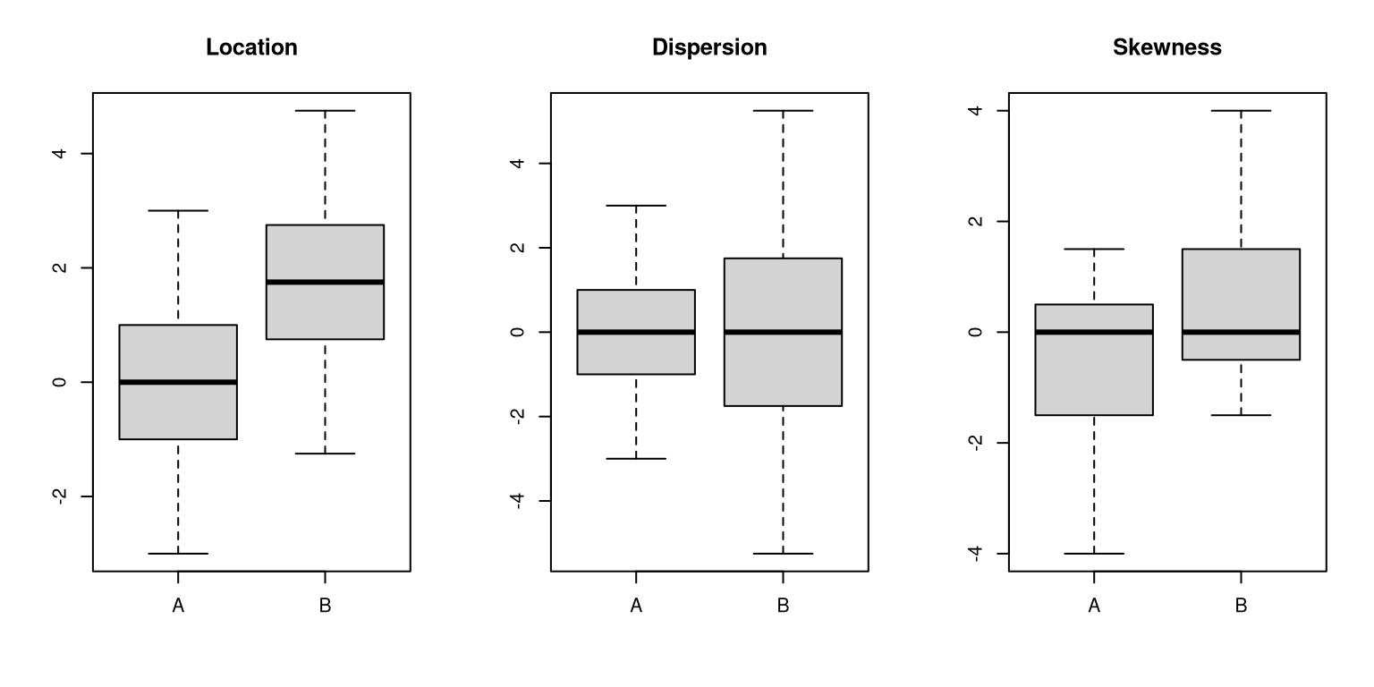
- \(H_1:\) At least one sample comes from another distributions (i.e., differs in some way such as location, dispersion, or skewness).
Idea: Although the distributions often differ in more than one of these properties, it is in principle possible that only one of location, dispersion, or skewness differs while the other properties are the same (see below). While location differences are of most interest in many applications, also dispersion differences may be of interest (e.g., when comparing different techniques to measure measurement techniques for a certain element in a chemical compound) or skewness differences (e.g., when assessing the risk in different financial products).
Initially: Compare two samples for location differences.
Data: Myopic loss aversion (MLA) experiment.
##    invest      gender male     age treatment grade arrangement
## 1 70.0000 female/male  yes 11.7533      long   6-8        team
## 2 28.3333 female/male  yes 12.0866      long   6-8        team
## 3 50.0000 female/male  yes 11.7950      long   6-8        team
## 4 50.0000        male  yes 13.7566      long   6-8        team
## 5 24.3333 female/male  yes 11.2950      long   6-8        team
## 6 83.0000        male  yes 11.8366      long   6-8        team
Here: Consider dependence of the main outcome variable invest on the experimental factor arrangement (single vs. team).
Group-wise statistics:
| Single | Team | Overall | |
|---|---|---|---|
| \(n\) | 385 | 185 | 570 |
| \(\overline y\) | 45.0 | 61.5 | 50.4 |
| \(Q_{0.5}\) | 44.4 | 62.7 | 50.0 |
| \(s\) | 26.2 | 24.5 | 26.8 |
| \(\mathit{IQR}\) | 40.0 | 34.3 | 40.0 |
| Min | 0 | 0 | 0 |
| Max | 100 | 100 | 100 |
9.3 Location differences
Intuitive: To assess whether invest depends on the explanatory variable arrangement, the empirical mean investment in the two arrangements can be compared: \(45.0\) (single) and \(61.5\) (team).
Simple idea: To test for significant location differences, the differences of the means (\(45.0 - 61.5 = -16.5\)) can be used and standardized by a suitable standard error.
Formally: Consider two independent random variables \(Y_A\) and \(Y_B\). The corresponding expectations are \(\text{E}(Y_A) = \mu_A\) and \(\text{E}(Y_B) = \mu_B\), respectively.
Question: Are the expectations \(\mu_A\) and \(\mu_B\) the same?
Answer: Test
\[\begin{array}{lrcl} H_0: & \mu_A & = & \mu_B \\ H_1: & \mu_A & \neq & \mu_B \end{array}\]based on empirical data.
Remark: Initially we assume that the two variable may only differ in location, i.e., other moments of the distributions are the same. In particular, the variances are equal \(\text{V}(Y_A) = \text{V}(Y_B) = \sigma^2\).
Notation:
- \(n_A\) observations from \(Y_A\) with realizations \(y_{A,1}, \dots, y_{A,n_A}\).
Corresponding empirical mean \(\overline y_A\) and variance \(s_A^2\). - \(n_B\) observations from \(Y_B\) with realizations \(y_{B,1}, \dots, y_{B,n_B}\).
Corresponding empirical mean \(\overline y_B\) and variance \(s_B^2\).
Intuitive: Consider difference of empirical means \(\overline y_A - \overline y_B\).
Question: How large is the random variation of this difference?
Answer:
\[\begin{eqnarray*} \text{E}(\overline Y_A - \overline Y_B) & = & \mu_A - \mu_B \\ \text{V}(\overline Y_A - \overline Y_B) & = & \frac{\text{V}(Y_A)}{n_A} + \frac{\text{V}(Y_B)}{n_B} \; = \; \frac{n_A + n_B}{n_A \cdot n_B} \cdot \sigma^2 \end{eqnarray*}\]
9.4 Two-sample \(t\)-test
Test statistic: Scaled difference of the means
\[ t \quad = \quad \frac{\overline y_A - \overline y_B}{\widehat{\mathit{SD}}}. \]
Scaling: Estimate the standard deviation \(\sigma^2\) of the observations and plug it into the standard deviation for the difference of the means.
\[ \widehat{\mathit{SD}} \quad = \quad \sqrt{ \frac{n_A + n_B}{n_A \cdot n_B} \cdot \frac{(n_A - 1) \cdot s_A^2 + (n_B - 1) \cdot s_B^2}{n_A + n_B - 2} }. \]
Null distribution: Under \(H_0\) and assuming both \(Y_A\) and \(Y_B\) are normally distributed, this \(t\)-statistic is \(t\)-distributed with \(n-2\) degrees of freedom. For increasing \(n-2\) the \(t\)-distribution converges to a standard normal distribution.
Central limit theorem (CLT): For any distribution of \(Y_A\) and \(Y_B\) the statistic \(t\) is asymptotically standard normal under \(H_0\).
Critical values: The 2-sided critical values at significance level \(\alpha\) are \(\pm t_{n-2; 1 - \alpha/2}\), i.e., \(\pm\) the \((1 - \alpha/2)\) quantile of the \(t_{n-2}\) distribution. Rule of thumb: The critical values at the \(\alpha = 0.05\) level are approximately \(t_{n-2; 0.975} \approx 2\).
Test decision: Reject the null hypothesis if \(|t| > t_{n-2; 1 - \alpha/2}\).
\(p\)-value: Analogously compute the corresponding \(p\)-value \(p = P_{H_0}(|T| > |t|)\). Reject the null hypothesis if \(p < \alpha\).
Confidence interval: The level \(\alpha\) confidence interval for the true difference in expectations \(\Delta = \mu_A - \mu_B\) can also be computed based on the critical values.
\[\begin{equation*} \left[ \hat \Delta ~-~ t_{n-2; 1 - \alpha/2} \cdot \widehat{\mathit{SD}} ~;~~ \hat \Delta ~+~ t_{n-2; 1 - \alpha/2} \cdot \widehat{\mathit{SD}} \right] \end{equation*}\]
Example: Assume that the difference of empirical means is \(\hat \Delta = 3\) and the estimated standard deviation is \(\widehat{\mathit{SD}} = 2\). Then \(t = 3/2 = 1.5\). Thus, the null hypothesis cannot be rejected at 5% level.
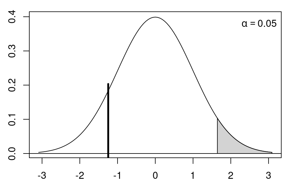
Illustration: Differences of mean investment between single players and teams.
| Single | Team | |
|---|---|---|
| \(n\) | 385 | 185 |
| \(\overline y\) | 45.0 | 61.5 |
| \(s\) | 26.2 | 24.5 |
Test: Assess equality of mean investments at 5% significance level.
Test statistic:
\[\begin{eqnarray*} \widehat{\mathit{SD}} & = & \sqrt{ \frac{385 + 185}{385 \cdot 185} \cdot \frac{(385 - 1) \cdot 26.2^2 + (185 - 1) \cdot 24.5^2}{385 + 185 - 2} } \\ & = & 2.30 \\ t & = & \frac{45.0 - 61.5}{ 2.30} \\ & = & -7.19. \end{eqnarray*}\]
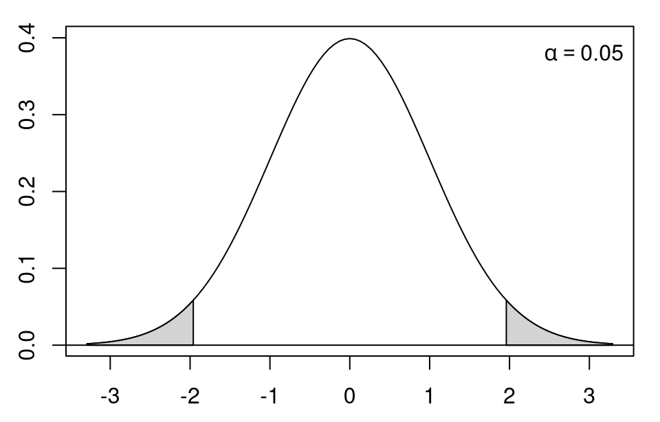
Thus, this is much smaller than \(t_{568; 0.025} = -1.96\).
Interpretation: Single players invest significantly less than teams.
In R:
##
##  Two Sample t-test
##
## data:  invest by arrangement
## t = -7.194, df = 568, p-value = 1.99e-12
## alternative hypothesis: true difference in means between group single and group team is not equal to 0
## 95 percent confidence interval:
##  -21.0466 -12.0193
## sample estimates:
## mean in group single   mean in group team
##              45.0124              61.5453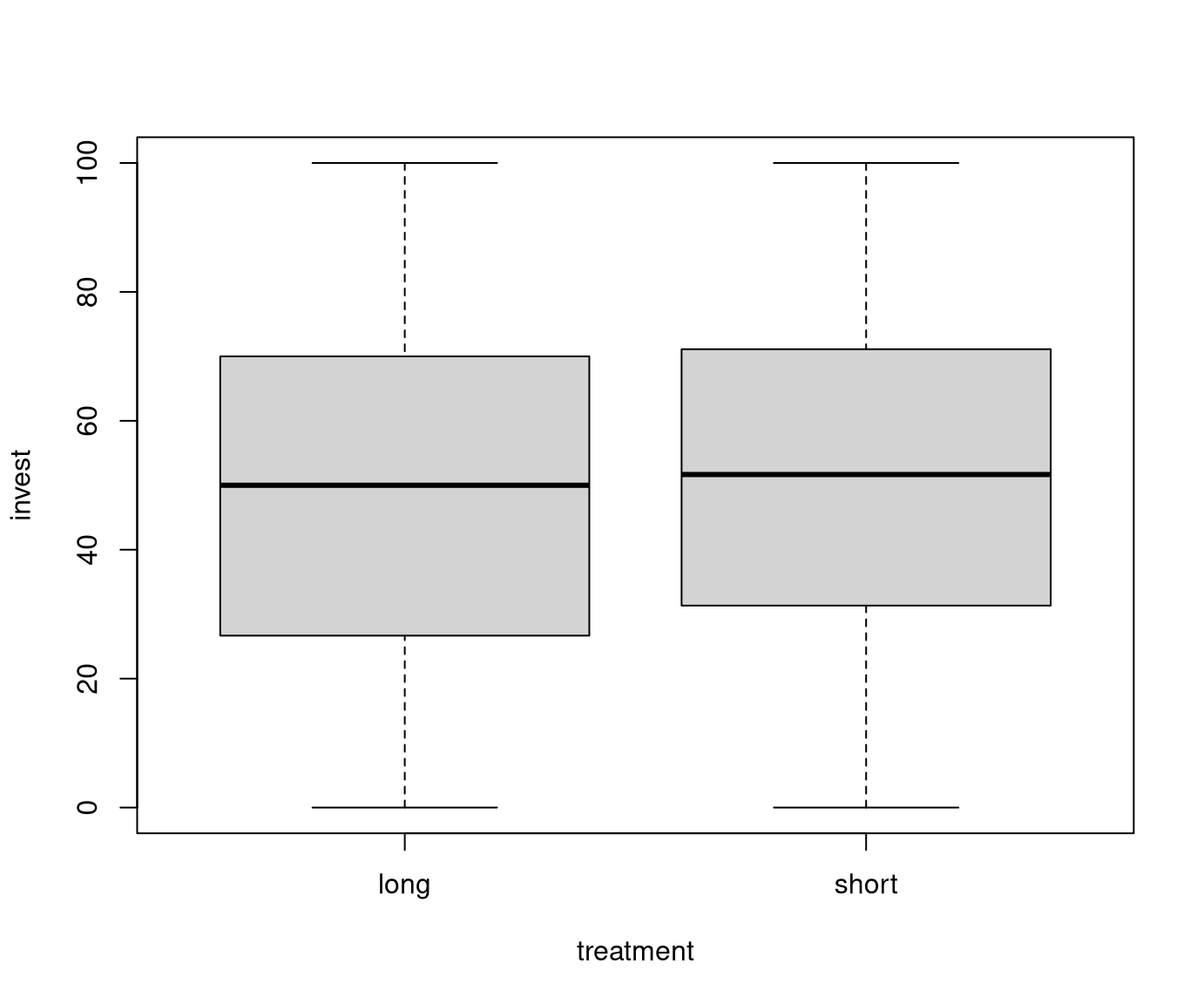
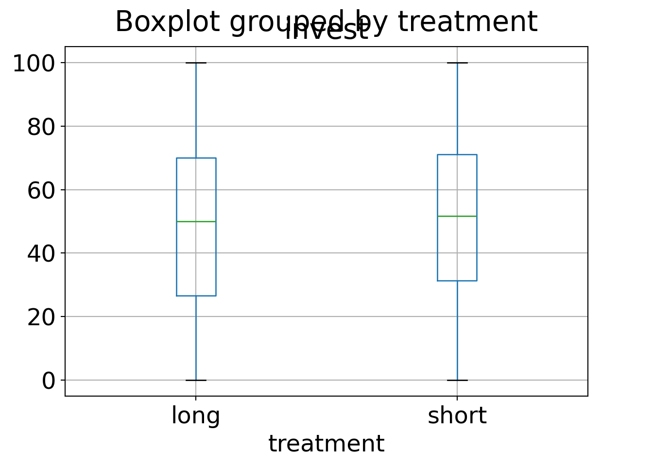
Illustration: Differences of mean investment between long and short treatment.
| Long | Short | |
|---|---|---|
| \(n\) | 285 | 285 |
| \(\overline y\) | 49.0 | 51.8 |
| \(s\) | 26.7 | 26.9 |
Test: Can we show at 5% significance level that investments are lower in the short treatment than in the long treatment?
Test statistic:
\[\begin{eqnarray*} \widehat{\mathit{SD}} & = & \sqrt{ \frac{285 + 285}{285 \cdot 285} \cdot \frac{284 \cdot 26.7^2 + 284 \cdot 26.9^2}{568} } \\ & = & 2.25 \\ t & = & \frac{49.0 - 51.8}{ 2.25} \\ & = & -1.25. \end{eqnarray*}\]
Thus, this is not greater than \(t_{568; 0.05} = -1.65\).
Interpretation: Investments in the short treatment are not significantly lower.
In R:
##
##  Two Sample t-test
##
## data:  invest by treatment
## t = -1.269, df = 568, p-value = 0.897
## alternative hypothesis: true difference in means between group long and group short is greater than 0
## 95 percent confidence interval:
##  -6.54609      Inf
## sample estimates:
##  mean in group long mean in group short
##             48.9544             51.8023
Question: How to estimate the standard deviation when the variances \(\text{V}(Y_A) \neq \text{V}(Y_B)\)?
Answer: Compute the \(t\)-statistic with
\[ \widehat{\mathit{SD}} \quad = \quad \sqrt{ \frac{s_A^2}{n_A} + \frac{s_B^2}{n_B} }. \]
Null distribution: Under \(H_0\) the resulting \(t\)-statistic is approximately \(t_\delta\)-distribution with degrees of freedom
\[ \delta \quad = \quad \frac{% \left( \frac{s_A^2}{n_A} + \frac{s_B^2}{n_B} \right)^2 }{% \frac{s_A^4}{n_A^2 (n_A - 1)} + \frac{s_B^4}{n_B^2 (n_B - 1)} }. \]
Name: Welch \(t\)-test.
In R:
##
##  Welch Two Sample t-test
##
## data:  invest by arrangement
## t = -7.371, df = 386.6, p-value = 1.04e-12
## alternative hypothesis: true difference in means between group single and group team is not equal to 0
## 95 percent confidence interval:
##  -20.9431 -12.1228
## sample estimates:
## mean in group single   mean in group team
## 45.0124 61.5453##
## Welch Two Sample t-test
##
## data: invest by treatment
## t = -1.269, df = 567.9, p-value = 0.897
## alternative hypothesis: true difference in means between group long and group short is greater than 0
## 95 percent confidence interval:
## -6.5461 Inf
## sample estimates:
## mean in group long mean in group short
## 48.9544 51.80239.5 Tutorial
For illustrating various 2-sample questions, data from an economic experiment
on myopic loss aversion MLA is used (Glätzle-Rützler, Sutter, Zeileis 2015.
No Myopic Loss Aversion in Adolescents? - An Experimental Note,
Journal of Economic Behavior & Organization, 111, 169-176).
The pupils participating in this experiment could invest in a lottery with
positive expectation over nine rounds. The risk-neutral choice would be to
always invest 100% of the points possible. However, due to risk aversion
or loss aversion many subjects typically invest less. The main research
question in this experiment, however, is whether this loss aversion effect
is enhanced when investments are made by short-term rather than long-term
decisions (myopia). The data set can be downloaded as MLA.csv or MLA.rda.
9.5.1 Setup
R
##    invest      gender male     age treatment grade arrangement
## 1 70.0000 female/male  yes 11.7533      long   6-8        team
## 2 28.3333 female/male  yes 12.0866      long   6-8        team
## 3 50.0000 female/male  yes 11.7950      long   6-8        team
Python
# Make sure that the required libraries are installed.
# Import the necessary libraries and classes:
import pandas as pd
import numpy as np
from matplotlib import pyplot as plt
import seaborn as sns

pd.set_option("display.precision", 4) # Set display precision to 4 digits in pandas and numpy.
# Load dataset
MLA = pd.read_csv("MLA.csv", index_col=False, header=0)
# Preview the first 5 lines of the loaded data
MLA.head()## invest gender male age treatment grade arrangement
## 0 70.0000 female/male yes 11.7533 long 6-8 team
## 1 28.3333 female/male yes 12.0866 long 6-8 team
## 2 50.0000 female/male yes 11.7950 long 6-8 team
## 3 50.0000 male yes 13.7566 long 6-8 team
## 4 24.3333 female/male yes 11.2950 long 6-8 team9.5.2 2 samples: Exploratory analysis
The dependent variable is invest, the average invested points across all 9 rounds.
The main treatment is whether the players could change investment decisions
in every round (short) or only for three rounds in a row (long).
Another important factor that was varied in the experiment is the
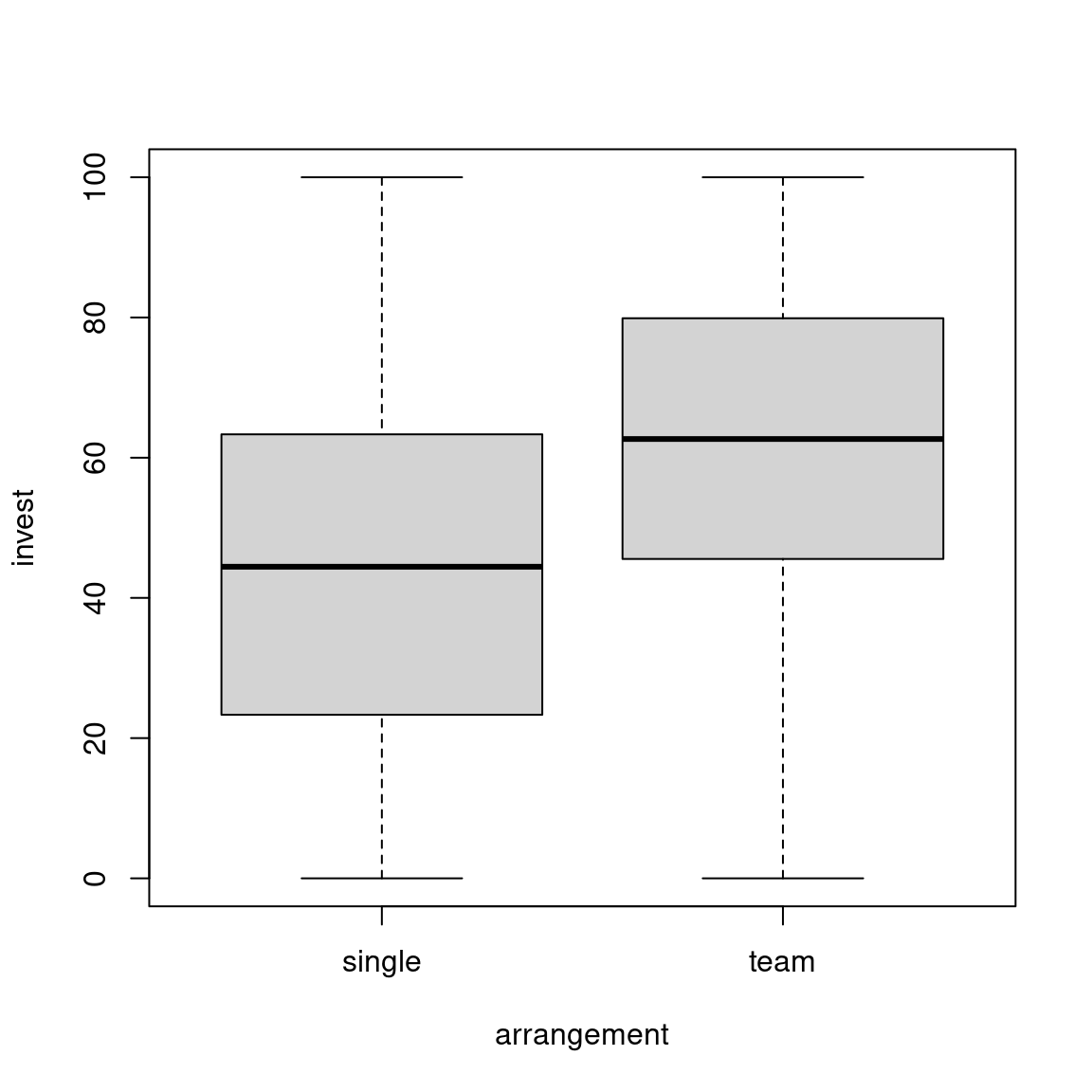
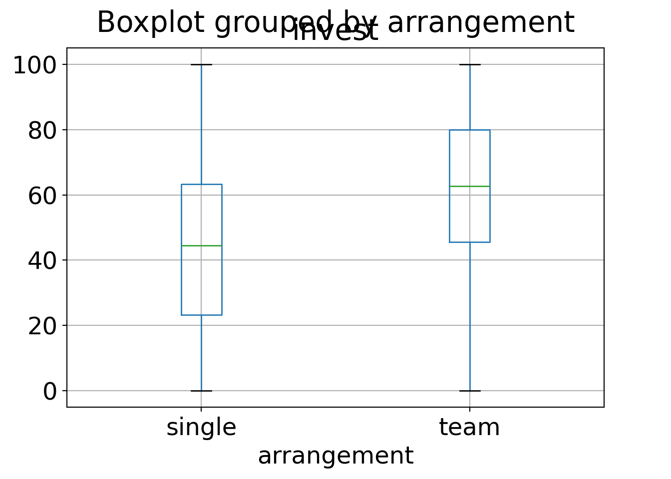
arrangement, i.e., whether investments were made by single players or
by teams of two. Both of these experimental factors will be used in the
following to create a 2-sample setup.
Further explanatory variables that will be used later on are the
gender of the (team of) player(s), an indicator whether
(at least one of) the player(s) (in the team) was male, the (average)
age, and the school grade (6-8 vs. 10-12).
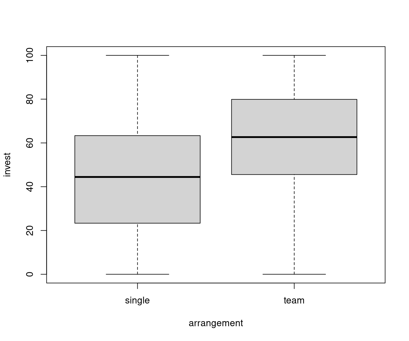
An exploratory visualization using parallel boxplots shows that the arrangement
appears to have an clear effect on invest (with teams behaving more rational
than single players) while the main treatment seems to have no effect at all
(i.e., the pupils do not seem to be affected by myopia).


We obtain the corresponding 2-sample statistics (first only means in both arrangement groups):
Obtain all summary statistics shown in the lecture slides:
R
In R, we could employ repeated tapply() calls. Or, alternatively, we could put together a small
function that computes all the summary statistics in one vector:
mystats <- function(x) c(n = length(x), mean = mean(x),
  median = median(x), sd = sd(x), iqr = IQR(x), min = min(x), max = max(x))
This can then be applied to both single and team players as well as to the entire sample:
tab <- tapply(MLA$invest, MLA$arrangement, mystats)
cbind(
  Single = tab$single,
  Team = tab$team,
  All = mystats(MLA$invest)
)
## Single Team All
## n 385.0000 185.0000 570.0000
## mean 45.0124 61.5453 50.3784
## median 44.4444 62.6667 50.0000
## sd 26.2414 24.4932 26.8094
## iqr 40.0000 34.3333 40.0000
## min 0.0000 0.0000 0.0000
## max 100.0000 100.0000 100.0000Python
We obtain many of the summary statistics from the describe() function.
##              count     mean      std  min      25%      50%      75%    max
## arrangement
## single       385.0  45.0124  26.2414  0.0  23.3333  44.4444  63.3333  100.0
## team         185.0  61.5453  24.4932  0.0  45.5556  62.6667  79.8889  100.0
To obtain all summary statistics shown in the lecture slides, we could employ the aggregation agg() function.
from scipy.stats import iqr

# Compute summary statistics for each group (single and team)
tab = MLA.groupby("arrangement")["invest"].agg(n=len,
                                               mean=np.mean,
                                               median=np.median,
                                               sd=np.std,
                                               iqr=iqr,
                                               min=min,
                                               max=max)
## <string>:3: FutureWarning: The provided callable <function mean at 0x7f43797c8d60> is currently using SeriesGroupBy.mean. In a future version of pandas, the provided callable will be used directly. To keep current behavior pass the string "mean" instead.
## <string>:3: FutureWarning: The provided callable <function median at 0x7f4365efc400> is currently using SeriesGroupBy.median. In a future version of pandas, the provided callable will be used directly. To keep current behavior pass the string "median" instead.
## <string>:3: FutureWarning: The provided callable <function std at 0x7f43797c8ea0> is currently using SeriesGroupBy.std. In a future version of pandas, the provided callable will be used directly. To keep current behavior pass the string "std" instead.
## <string>:3: FutureWarning: The provided callable <built-in function min> is currently using SeriesGroupBy.min. In a future version of pandas, the provided callable will be used directly. To keep current behavior pass the string "min" instead.
## <string>:3: FutureWarning: The provided callable <built-in function max> is currently using SeriesGroupBy.max. In a future version of pandas, the provided callable will be used directly. To keep current behavior pass the string "max" instead.## n mean median sd iqr min max
## arrangement
## single 385 45.0124 44.4444 26.2414 40.0000 0.0 100.0
## team 185 61.5453 62.6667 24.4932 34.3333 0.0 100.0Analogously, we could obtain 2-sample statistics for invest grouped by treatment.
9.5.3 2-sample \(t\)-test
The classical parametric test for assessing the null hypothesis of equal distributions against location differences is the 2-sample \(t\)-test. Assuming both subsamples come from normal distributions with the same variance reduces null hypothesis and alternative to: \(\mu_A = \mu_B\) vs. \(\mu_A \neq \mu_B\).
R
This \(t\)-test can be carried out with t.test() and options var.equal = TRUE. Applying this to the MLA data
shows that there is a highly-significant difference between single players and teams
regarding the level of investments (or degree of loss aversion):
##
##  Two Sample t-test
##
## data:  invest by arrangement
## t = -7.194, df = 568, p-value = 1.99e-12
## alternative hypothesis: true difference in means between group single and group team is not equal to 0
## 95 percent confidence interval:
##  -21.0466 -12.0193
## sample estimates:
## mean in group single   mean in group team
##              45.0124              61.5453
Python
Perform a 2-sample \(t\)-test.
from statsmodels.stats.weightstats import ttest_ind

single = MLA[MLA['arrangement']=="single"]['invest']
team = MLA[MLA['arrangement']=="team"]['invest']

ttest = ttest_ind(x1=single, x2=team, alternative="two-sided", usevar="pooled")
print("t = {:.1f}, p-value = {:.1g}, df = {:.0f}".format(ttest[0],ttest[1],ttest[2]))
## t = -7.2, p-value = 2e-12, df = 568In addition to the two-sided alternative \(\mu_A \neq \mu_B\) it is possible to
also assess the one-sided alternatives \(\mu_A > \mu_B\) (alternative = "greater")
and \(\mu_A < \mu_B\) (alternative = "less").
This is useful for assessing the main treatment effect in the MLA data. Economic
theory would suggest that mean investments should be greater in the long
condition compared to the short condition. The corresponding \(t\)-test can be
conducted with:
R
##
##  Two Sample t-test
##
## data:  invest by treatment
## t = -1.269, df = 568, p-value = 0.897
## alternative hypothesis: true difference in means between group long and group short is greater than 0
## 95 percent confidence interval:
##  -6.54609      Inf
## sample estimates:
##  mean in group long mean in group short
##             48.9544             51.8023
Python
long = MLA[MLA['treatment']=="long"]['invest']
short = MLA[MLA['treatment']=="short"]['invest']

ttest = ttest_ind(x1=long, x2=short, alternative="larger", usevar="pooled")
print("t = {:.1f}, p-value = {:.1g}, df = {:.0f}".format(ttest[0],ttest[1],ttest[2]))
## t = -1.3, p-value = 0.9, df = 568This shows clearly that this cannot be significant for this data because the empirical average investment in the long condition is already lower than in the short condition.
Finally, the assumption of equal variances can be given up:
R
By using var.equal = FALSE which is the default in t.test().
##
##  Welch Two Sample t-test
##
## data:  invest by arrangement
## t = -7.371, df = 386.6, p-value = 1.04e-12
## alternative hypothesis: true difference in means between group single and group team is not equal to 0
## 95 percent confidence interval:
##  -20.9431 -12.1228
## sample estimates:
## mean in group single   mean in group team
## 45.0124 61.5453##
## Welch Two Sample t-test
##
## data: invest by treatment
## t = -1.269, df = 567.9, p-value = 0.897
## alternative hypothesis: true difference in means between group long and group short is greater than 0
## 95 percent confidence interval:
## -6.5461 Inf
## sample estimates:
## mean in group long mean in group short
## 48.9544 51.8023Python
By using usevar=unequal (usevar=pooled is the default).
ttest = ttest_ind(x1=single, x2=team, alternative="two-sided", usevar="unequal")
print("t = {:.1f}, p-value = {:.1g}, df = {:.0f}".format(ttest[0],ttest[1],ttest[2]))
## t = -7.4, p-value = 1e-12, df = 387ttest = ttest_ind(x1=long, x2=short, alternative="larger", usevar="unequal")
print("t = {:.1f}, p-value = {:.1g}, df = {:.0f}".format(ttest[0],ttest[1],ttest[2]))## t = -1.3, p-value = 0.9, df = 568Note that then the \(t\)-distribution only holds approximately under the null hypothesis, even if the 2 samples come from normal distributions. This is known as the Welch approximation and the corresponding test as Welch 2-sample \(t\)-test.
For the MLA data setting var.equal = FALSE or TRUE in R or usevar=unequal or pooled in Python does not make much difference because variances across both arrangement and treatment are rather homogeneous anyway.