Chapter 12 Independence tests

12.1 Robust tests

12.1.1 Robust statistics

\(t\)-test: As the mean is no robust measure of location (i.e., can change arbitrarily based on a single observation), the \(t\)-statistic is also not robust.

Robust alternatives:

• Median difference: The median is a robust measure of location.
• Difference of trimmed means: Omit a certain proportion of the most extreme observations prior to computing means.
• Rank sums: Compute ranks of all observations in the pooled sample and compute the rank sum of one of the samples.

All of these statistics are robust in the sense that a single outlier has limited influence on the statistic only. Hence, the power is not so affected by outliers compared to classical parametric statistics.

12.1.2 Rank tests

In practice: Although less intuitive than, e.g., the median difference, rank sums are the most frequently-used robust statistics.

In part this is dues to historic reasons.

• Historically: Rank tests were popular because the permutation principle could be applied easily (without having access to modern computers).
• Today: Rank tests are applied due to their robustness properties against heavy tails or outliers (i.e., not due to being “distribution-free”).

Example: The most commonly-used rank test is the Wilcoxon rank sum test or Wilcoxon-Mann-Whitney test.

12.1.3 Wilcoxon-Mann-Whitney test

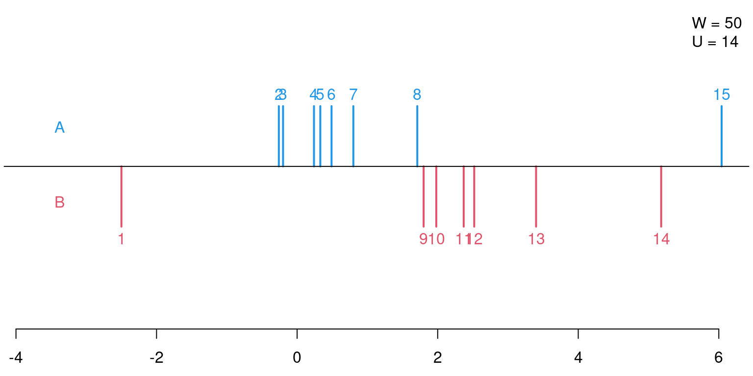
Test statistics: Compute the ranks \(R_i\) in the pooled sample of all \(n = n_A + n_B\) observations. Employ the sum of the ranks in the \(A\) sample as the test statistic (Wilcoxon statistic): \[ W \quad = \quad \sum_{i = 1}^{n_A} R_i. \]

An equivalent test statistic is given by the Mann-Whitney \(U\)-statistic: \[ U \quad = \quad W - n_A \cdot (n_A + 1)/2. \] This is what wilcox.test() computes in base R.

Null distribution: Various algorithms can evaluate the permutation distribution exactly (without explicitly computing all possible permutations).

In R:

wilcox.test(y ~ x, data = dat0)

## 
##  Wilcoxon rank sum exact test
## 
## data:  y by x
## W = 14, p-value = 0.121
## alternative hypothesis: true location shift is not equal to 0

t.test(y ~ x, data = dat0)

## 
##  Welch Two Sample t-test
## 
## data:  y by x
## t = -0.8399, df = 12.17, p-value = 0.417
## alternative hypothesis: true difference in means between group A and group B is not equal to 0
## 95 percent confidence interval:
##  -3.45869  1.53191
## sample estimates:
## mean in group A mean in group B 
##         1.14375         2.10714

In R: With coin.

wilcox_test(y ~ x, data = dat0, distribution = "exact")

## 
##  Exact Wilcoxon-Mann-Whitney Test
## 
## data:  y by x (A, B)
## Z = -1.62, p-value = 0.121
## alternative hypothesis: true mu is not equal to 0

Remarks:

• The coin package standardizes the test statistic in a similar way as the \(t\)-test. This does not affect the \(p\)-value though.
• The algorithm for the exact permutation distribution in wilcox_test() works also in the presence of ties, i.e., when the same \(Y\)-value occurs in both the \(A\) and \(B\) sample.
• However, the classical algorithm for the permutation \(p\)-value, as implemented in wilcox.test(), only works exactly without such ties.

Computing the \(U\)-statistic by hand:

dat0

##        y x
## 1  -2.50 B
## 2  -0.26 A
## 3  -0.20 A
## 4   0.24 A
## 5   0.33 A
## 6   0.49 A
## 7   0.80 A
## 8   1.71 A
## 9   1.80 B
## 10  1.98 B
## 11  2.37 B
## 12  2.52 B
## 13  3.40 B
## 14  5.18 B
## 15  6.04 A

\[\begin{eqnarray*} W & = & 2 + 3 + 4 + 5 + 6 + 7 + 8 + 15 \\ & = & 50 \\ U & = & W - n_A \cdot (n_A + 1)/2 \\ & = & 50 - 8 \cdot 9/2 \\ & = & 14 \end{eqnarray*}\]

Example: Dependence of invest on arrangement or treatment, respectively, in the MLA data.

wilcox.test(invest ~ arrangement, data = MLA)

## 
##  Wilcoxon rank sum test with continuity correction
## 
## data:  invest by arrangement
## W = 22858, p-value = 4.24e-12
## alternative hypothesis: true location shift is not equal to 0

wilcox.test(invest ~ treatment, data = MLA)

## 
##  Wilcoxon rank sum test with continuity correction
## 
## data:  invest by treatment
## W = 38238, p-value = 0.227
## alternative hypothesis: true location shift is not equal to 0

12.1.4 Efficiency differences

Efficiency: A test is more efficient than another when a lower sample size is necessary to obtain the same power.

For the 2-sample problem:

• If the variables \(Y_A\) and \(Y_B\) are indeed normally distributed, then the exact \(t\)-test is the most efficient for detecting location differences. Many robust tests (like the Wilcoxon-Mann-Whitney test), however, are almost as efficient.
• If \(Y_A\) and \(Y_B\) are non-normal, the \(t\)-test can become very inefficient, yielding misleading results. In contrast, many robust tests have good efficiency for a broad range of potential distributions.

12.1.5 Robust Kruskal-Wallis analysis of variance

\(k\)-sample problem: Employ a type of analysis of variance based on the ranks \(R_{ij}\) of observation \(i\) in sample \(j\) (Kruskal-Wallis test).

\[ K \quad = \quad (N - 1) ~ \frac{% \sum\limits_{j = 1}^k n_j (\overline R_j - \overline R)^2 }{% \sum\limits_{j = 1}^k \sum\limits_{i = 1}^{n_j} (R_{ij} - \overline R)^2 }, \]

where \(\overline R\) and \(\overline R_j\) are the average ranks overall and in sample \(j\), respectively. \(N = n_1 + n_2 + \dots + n_k\) is the overall sample size

Null distribution: Permutation distribution (directly computed from suitable algorithms).

kruskal.test(invest ~ gender, data = MLA)

## 
##  Kruskal-Wallis rank sum test
## 
## data:  invest by gender
## Kruskal-Wallis chi-squared = 52.68, df = 2, p-value = 3.64e-12

12.2 Correlation tests

12.2.1 Correlation of two quantitative variables

Question: Is there a (significant) correlation between two quantitative variables \(X\) and \(Y\)?

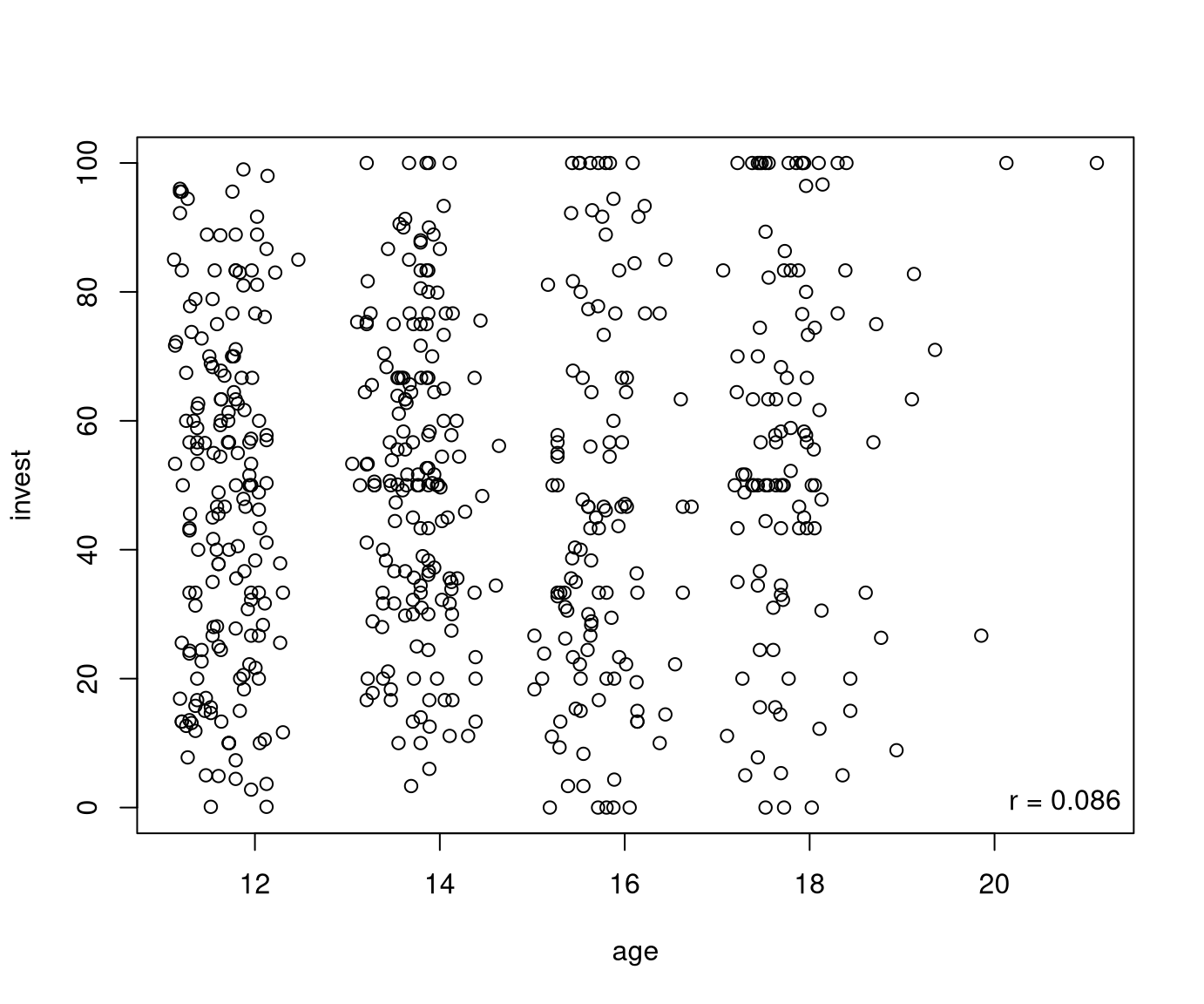
Example: Dependence of age on invest in the MLA data.

Measure of correlation: Pearson product-moment correlation coefficient. \[ r \quad = \quad \frac{% \sum\limits_{i = 1}^n (x_i - \overline x) (y_i - \overline y) }{% \sqrt{\sum\limits_{i = 1}^n (x_i - \overline x)^2 \sum\limits_{i = 1}^n (y_i - \overline y)^2} } \]

Test statistic: Standardized correlation.

\[ t \quad = \quad \frac{r}{\sqrt{\frac{1 - r^2}{n - 2}}} \]

Null distribution: Under the null distribution and under normality the \(t\) statistic is \(t\)-distributed with \(n-2\) degrees of freedom. It is asymptotically normally distributed. The permutation distribution can be easily simulated.

In R:

cor.test(~ age + invest, data = MLA, method = "pearson")

## 
##  Pearson's product-moment correlation
## 
## data:  age and invest
## t = 2.062, df = 568, p-value = 0.0397
## alternative hypothesis: true correlation is not equal to 0
## 95 percent confidence interval:
##  0.00408678 0.16712570
## sample estimates:
##       cor 
## 0.0861832

independence_test(invest ~ age, data = MLA, distribution = approximate(10000))

## 
##  Approximative General Independence Test
## 
## data:  invest by age
## Z = 2.056, p-value = 0.0384
## alternative hypothesis: two.sided

Robust alternatives: Robust correlation coefficients.

• Spearman’s \(\varrho\): Based on Pearson correlation coefficient based on rank-transformed variables.
• Kendall’s \(\tau\): Based on so-called concordances, i.e., observations where both \((x_i - \overline x)\) and \((y_i - \overline y)\) have the same sign.

Tests: For both correlation coefficients a test statistic with asymptotic normal distribution is available as well as algorithms for computing the exact permutation distribution.

In R:

cor.test(~ age + invest, data = MLA, method = "spearman")

## Warning in cor.test.default(x = mf[[1L]], y = mf[[2L]], ...): Cannot compute exact
## p-value with ties

## 
##  Spearman's rank correlation rho
## 
## data:  age and invest
## S = 28915923, p-value = 0.132
## alternative hypothesis: true rho is not equal to 0
## sample estimates:
##       rho 
## 0.0631607

independence_test(invest ~ age, data = MLA, distribution = approximate(10000),
  xtrafo = rank, ytrafo = rank)

## 
##  Approximative General Independence Test
## 
## data:  invest by age
## Z = 1.507, p-value = 0.135
## alternative hypothesis: two.sided

cor.test(~ age + invest, data = MLA, method = "kendall")

## 
##  Kendall's rank correlation tau
## 
## data:  age and invest
## z = 1.464, p-value = 0.143
## alternative hypothesis: true tau is not equal to 0
## sample estimates:
##       tau 
## 0.0413208

Interpretation: Investments of the pupils in the MLA data are only weakly correlated with their age. Tests based on the Pearson coefficient are just significant at 5% level while the robust alternatives are non-significant.

12.3 \(\chi^2\)-test for independence in contingency tables

12.3.1 Correlation of two qualitative variables

Question: Is there a (significant) correlation between two qualitative variables \(X\) and \(Y\)?

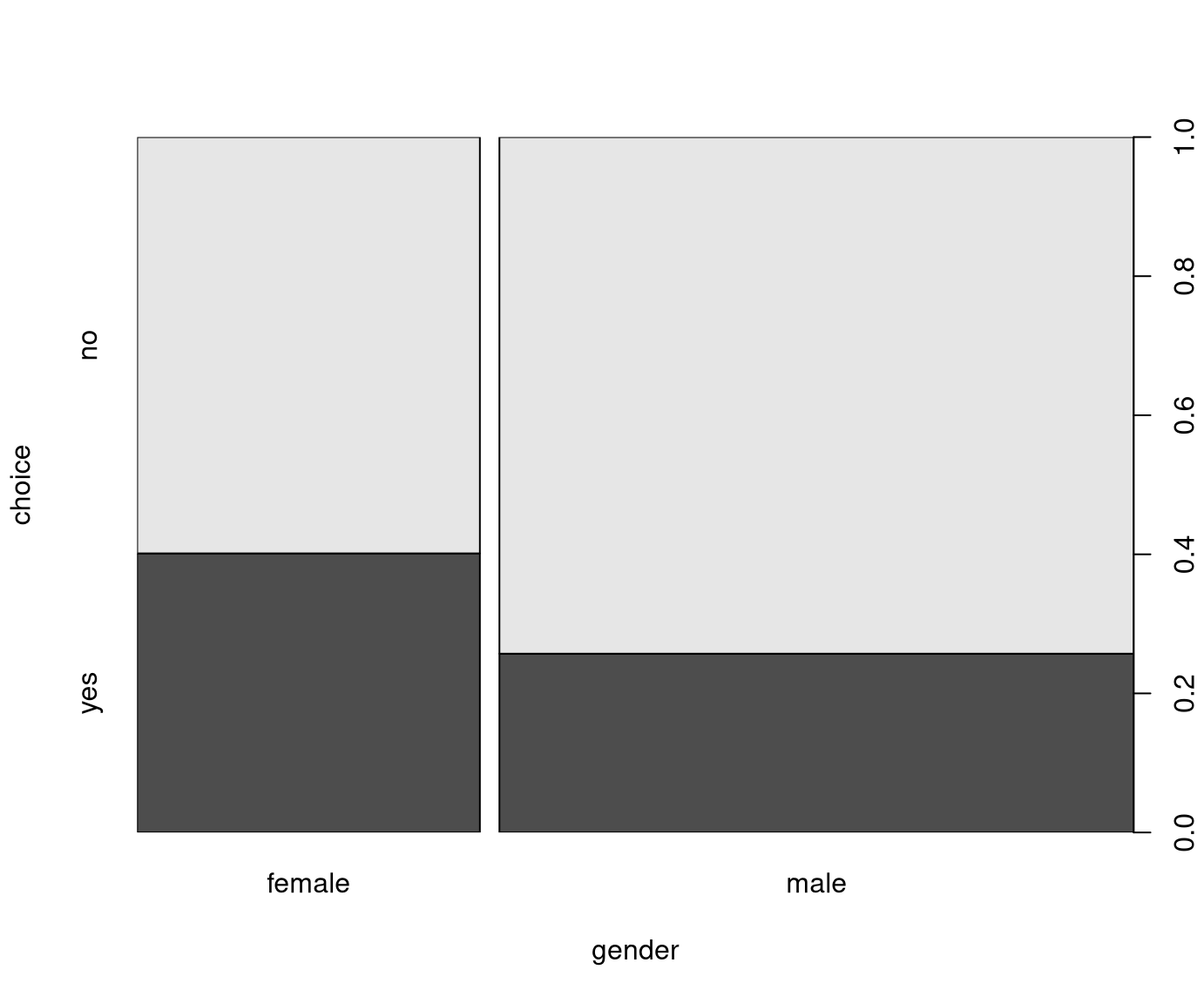
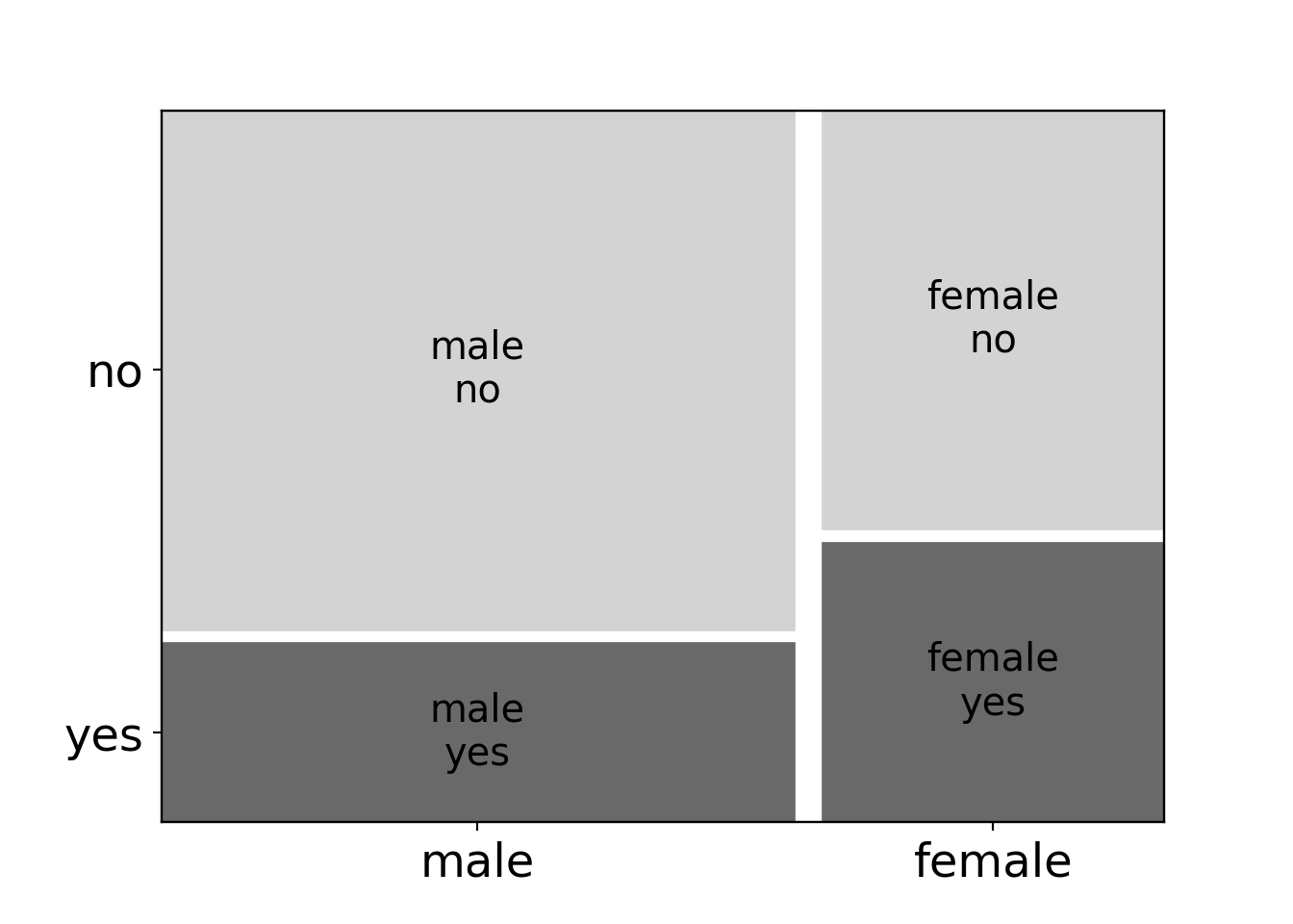
Example: Dependence of choice (purchase of the advertised art book) on gender in the BBBClub data.

Contingency table: With marginal sums.

Gender vs. choice	No	Yes	Sum
Women	\(273\)	\(183\)	\(456\)
Men	\(627\)	\(217\)	\(844\)
Sum	\(900\)	\(400\)	\(1300\)

Formally: Based on two categorical variables \(Y\) (with categories \(A_1, A_2, \dots, A_I\)) and \(X\) (with categories \(B_1, \dots, B_J\)).

Contingency table: The cells provide the observed frequencies \(O_{ij}\), indicating how often \(A_i \cap B_j\) were observed jointly in the sample.

	\(B_1\)	\(B_2\)	\(\cdots\)	\(B_J\)	Sum
\(A_1\)	\(O_{11}\)	\(O_{12}\)	\(\cdots\)	\(O_{1J}\)	\(O_{1+}\)
\(A_2\)	\(O_{21}\)	\(O_{22}\)	\(\cdots\)	\(O_{2J}\)	\(O_{2+}\)
\(\vdots\)	\(\vdots\)	\(\vdots\)	\(\ddots\)	\(\vdots\)	\(\vdots\)
\(A_I\)	\(O_{I1}\)	\(O_{I2}\)	\(\cdots\)	\(O_{IJ}\)	\(O_{I+}\)
Sum	\(O_{+1}\)	\(O_{+2}\)	\(\cdots\)	\(O_{+J}\)	\(O_{++} = n\)

12.3.2 Homogeneity vs. independence

Null hypothesis: Two ways to describe the lack of correlation.

• Homogeneity: The distribution of the dependent variable \(Y\) (here: choice) is homogeneous across the groups with respect to \(X\) (here: women and men).
• Independence: The variables \(Y\) and \(X\) are stochastically independent.

Equivalence: Both considerations lead to an assessment of the same quantities.

Formally: Homogeneity is given by

\[ \text{P}(A_i | B_j) \; = \; \text{P}(A_i). \]

Using the definition of conditional probabilities:

\[ \text{P}(A_i|B_j) \; = \; \frac{\text{P}(A_i \cap B_j)}{\text{P}(B_j)} \; = \; \text{P}(A_i). \]

Or:

\[ \text{P}(A_i \cap B_j) \; = \; \text{P}(A_i)\text{P}(B_j).\]

This is the definition of stochastic independence of \(A_i\) and \(B_j\).

12.3.3 Expected frequencies

Estimation: Under the null hypothesis of independence the probability for an observation in row \(i\) and column \(j\) is:

\[ \text{P}(A_i \cap B_j) = \text{P}(A_i) \cdot \text{P}(B_j). \]

The corresponding probabilities \(\text{P}(A_i)\) and \(\text{P}(B_j)\) can be estimated from the marginal relative frequencies:

\[ \text{P}(A_i) \approx \frac{O_{i+}}{n} \quad \mbox{and} \quad \text{P}(B_j) \approx \frac{O_{+j}}{n} \]

Thus: The expected frequencies \(\text{E}_{ij}\) in a sample of size \(n\) are

\[ n \cdot \text{P}(A_i \cap B_j) = n \cdot \text{P}(A_i) \cdot \text{P}(B_j) \approx n \cdot \frac{O_{i+}}{n} \cdot \frac{O_{+j}}{n} %% = \frac{O_{i+} \cdot O_{+j}} {n} = \text{E}_{ij}. \]

Result: The expected frequencies \(\text{E}_{ij}\) are the product of the corresponding marginal observed frequencies divided by the sample size.

\[ \text{E}_{ij} = \frac{O_{i+} \cdot O_{+j}}{n} \]

Example: Expected frequencies for the BBBClub data.

Gender vs. choice	No	Yes
Women	\(315.7\)	\(140.3\)
Men	\(584.3\)	\(259.7\)

12.3.4 \(\chi^2\)-test

Test statistic: To capture overall deviations between observed and expected frequencies across the entire table, the Pearson \(X^2\)-statistic is used:

\[ X^2 = \sum_{i=1}^I \sum_{j=1}^J \frac{(O_{ij} - \text{E}_{ij})^2}{\text{E}_{ij}}. \]

Example: BBBClub data.

\[ X^2 = \frac{(273 - 315.7)^2}{315.7} + \cdots + \frac{(217 - 259.7)^2}{259.7} = 28.901 \]

Additionally: The scaled deviations \((O_{ij} - \text{E}_{ij})/\sqrt{\text{E}_{ij}}\) from \(X^2\) can provide insights into the patterns of dependence in case of significant results.

Null distribution: Under the null hypothesis, \(X^2\) is asymptotically \(\chi^2\)-distributed with \((I-1) \cdot (J-1)\) degrees of freedom.

Continuity correction: The asymptotic approximation can be improved in fourfold tables when a continuity correction is included in the enumerator of \(X^2\): \((|O_{ij} - \text{E}_{ij}| - 0.5)^2\) (Yates correction).

Rule of thumb: The asymptotic approximation should not be used if the expected value in any cell is too small: \(\text{E}_{ij} < 5\).

Alternatively: Simulation of the permutation distribution.

In R:

tab <- xtabs(~ gender + choice, data = BBBClub)
chisq.test(tab)

## 
##  Pearson's Chi-squared test with Yates' continuity correction
## 
## data:  tab
## X-squared = 28.23, df = 1, p-value = 0.000000108

chisq.test(tab, correct = FALSE)

## 
##  Pearson's Chi-squared test
## 
## data:  tab
## X-squared = 28.9, df = 1, p-value = 0.0000000762

In R: With coin.

chisq_test(tab, distribution = approximate(10000))

## 
##  Approximative Pearson Chi-Squared Test
## 
## data:  choice by gender (female, male)
## chi-squared = 28.9, p-value <0.0001

Interpretation: All tests show that the choice decisions depend significantly on the gender in the BBBClub data. Women are more likely to purchase the advertised art book than men.

12.3.5 Fisher’s exact test

Remark: The exact test for dependence in contingency tables has a so-called hypergeometric distribution which can be easily evaluated in four-way tables (Fisher’s exact test).

In R: Also for higher-order contingency tables.

fisher.test(tab)

## 
##  Fisher's Exact Test for Count Data
## 
## data:  tab
## p-value = 0.000000113
## alternative hypothesis: true odds ratio is not equal to 1
## 95 percent confidence interval:
##  0.402220 0.663346
## sample estimates:
## odds ratio 
##   0.516571

12.4 Related methods

Parametric tests:

• Classical tests for quantitative dependent variables (\(t\)-test, \(F\)-test/ANOVA, Pearson correlation test) under the assumption of equal variances are special cases of the linear regression model.
• Part III: \(t\)-test and \(F\)-test/ANOVA in the linear regression model.

Permutation and rank tests:

• Broad variety of nonparametric tests for location and dispersion alternatives, etc.
• Van der Waerden, Mood, Ansari-Bradley, Fligner-Killeen, Cochran-Mantel-Haenszel, …

\(\chi^2\)-test:

• Log-linear models for multi-way contingency tables.
• Logistic regression for binary/multinomial/ordered dependent variables.
• Chapter 4: Binary logistic regression using quantitative and qualitative explanatory variables.

12.5 Tutorial

12.5.1 Setup

Load the MLA (MLA.csv, MLA.rda) and the BBBClub (BBBClub.csv, BBBClub.rda) data sets.

R

load("MLA.rda")
head(MLA, 3)

##    invest      gender male     age treatment grade arrangement
## 1 70.0000 female/male  yes 11.7533      long   6-8        team
## 2 28.3333 female/male  yes 12.0866      long   6-8        team
## 3 50.0000 female/male  yes 11.7950      long   6-8        team

load("../data/BBBClub.rda")

Python

# Make sure that the required libraries are installed.
# Import the necessary libraries and classes:
import pandas as pd 
import numpy as np
from matplotlib import pyplot as plt
import seaborn as sns
from scipy import stats
from r_functions import create

pd.set_option("display.precision", 4) # Set display precision to 4 digits in pandas and numpy.

# Load the MLA and BBBClub datasets
MLA = pd.read_csv("MLA.csv", index_col=False, header=0) 
BBBClub = pd.read_csv("BBBClub.csv", index_col=False, header=0) 

12.5.2 Robust rank tests

If the data in the 2 samples to be tests is very non-normal (i.e., not unimodal, symmetric, without outliers) then means are often not a good location measure because the mean can be biased in empirical samples. Consequently, the corresponding \(t\)-test is then suboptimal. In such situations it is usually better to employ a test statistic that is based on a robust location measure. The most popular robust tests in practice are the Wilcoxon-Mann-Whitney test in the 2-sample setup and the Kruskal-Wallis test in the \(k\)-sample setup.

R

Both are easily available in base R and compute the “exact” permutation distribution using fast recursion algorithms. For example, for the test of arrangement:

wilcox.test(invest ~ arrangement, data = MLA)

## 
##  Wilcoxon rank sum test with continuity correction
## 
## data:  invest by arrangement
## W = 22858, p-value = 4.24e-12
## alternative hypothesis: true location shift is not equal to 0

Python

Note: the function wilcoxon in scipy is the paired test which requires equal length. To perform two-sample Wilcoxon tests on vectors of data (Wilcoxon-Mann-Whitney test) use mannwhitneyu.

from scipy.stats import mannwhitneyu

(W, p) = mannwhitneyu(x=MLA[MLA['arrangement']=="single"]['invest'], y=MLA[MLA['arrangement']=="team"]['invest'], use_continuity=True, alternative='two-sided')
print("W = {:.0f}, p-value = {:.1g}".format(W, p))

## W = 22858, p-value = 4e-12

The test’s popularity stems from a time where it was not easily possible to sample 10,000 permutations on a computer while the fast recursion algorithms could be computed. This also explains why the rank-based tests are more widely-used than other tests, e.g., based on differences of medians or trimmed means, which might be more intuitive.

However, the recursion algorithms for computing the \(p\)-values only work exactly when there are no ties in the response across the samples (i.e., the same value of y occurs by chance in different subsamples with respect to x). In such a situation the coin package provides more refined algorithms that compute the exact \(p\)-values in the presence of ties. Alternatively, even if no exact \(p\)-value is available, the exact \(p\)-value can be approximated arbitrarily closely by drawing a large enough number of permutations.

R

library("coin")
wilcox_test(invest ~ arrangement, data = MLA, distribution = "exact")

## 
##  Exact Wilcoxon-Mann-Whitney Test
## 
## data:  invest by arrangement (single, team)
## Z = -6.929, p-value = 2.03e-12
## alternative hypothesis: true mu is not equal to 0

wilcox_test(invest ~ arrangement, data = MLA, distribution = approximate(10000))

## 
##  Approximative Wilcoxon-Mann-Whitney Test
## 
## data:  invest by arrangement (single, team)
## Z = -6.929, p-value <0.0001
## alternative hypothesis: true mu is not equal to 0

Python

For the setup of the coin package in Python, see Chapter 11.5.2

Note: the exact tests takes a while to finish!

wilcox_test = create("coin.R", "wilcox_test")
res = wilcox_test(formula="invest ~ arrangement", data="MLA.csv", distribution="exact")
print(res)

## {'method': 'Exact Wilcoxon-Mann-Whitney Test', 'data': 'invest by arrangement (single, team)', 'statistic': -6.9294, 'pvalue': 2.0279e-12, 'alternative': 'true mu is not equal to 0'}

res = wilcox_test(formula="invest ~ arrangement", data="MLA.csv", distribution=10000)
print(res)

## {'method': 'Approximative Wilcoxon-Mann-Whitney Test', 'data': 'invest by arrangement (single, team)', 'statistic': -6.9294, 'pvalue': 0, 'alternative': 'true mu is not equal to 0'}

For completeness we also show the 1-sided test result of investment by gender and the \(k\)-sample Kruskal-Wallis test.

R

In R, both are carried out by base R functions again.

wilcox.test(invest ~ treatment, data = MLA, alternative = "greater")

## 
##  Wilcoxon rank sum test with continuity correction
## 
## data:  invest by treatment
## W = 38238, p-value = 0.887
## alternative hypothesis: true location shift is greater than 0

kruskal.test(invest ~ gender, data = MLA)

## 
##  Kruskal-Wallis rank sum test
## 
## data:  invest by gender
## Kruskal-Wallis chi-squared = 52.68, df = 2, p-value = 3.64e-12

Python

(W, p) = mannwhitneyu(x=MLA[MLA['treatment']=="long"]['invest'], y=MLA[MLA['treatment']=="short"]['invest'], use_continuity=True, alternative='greater')
print("W = {:.0f}, p-value = {:.1g}".format(W, p))

## W = 38238, p-value = 0.9

from scipy.stats import kruskal

female = MLA[MLA['gender']=="female"]['invest']
fem_mal = MLA[MLA['gender']=="female/male"]['invest']
male = MLA[MLA['gender']=="male"]['invest']

stat, p = kruskal(female, fem_mal, male)
print("chi-squared = {:.0f}, p-value = {:.1g}".format(stat, p))

## chi-squared = 53, p-value = 4e-12

Kruskal-Wallis test with coin

kruskal_test = create("coin.R", "kruskal_test")
res = kruskal_test(formula="invest ~ gender", data="MLA.csv")
print(res)

## {'method': 'Asymptotic Kruskal-Wallis Test', 'data': 'invest by gender (female, female/male, male)', 'statistic': 52.6788, 'pvalue': 3.6386e-12}

12.5.3 Correlation tests

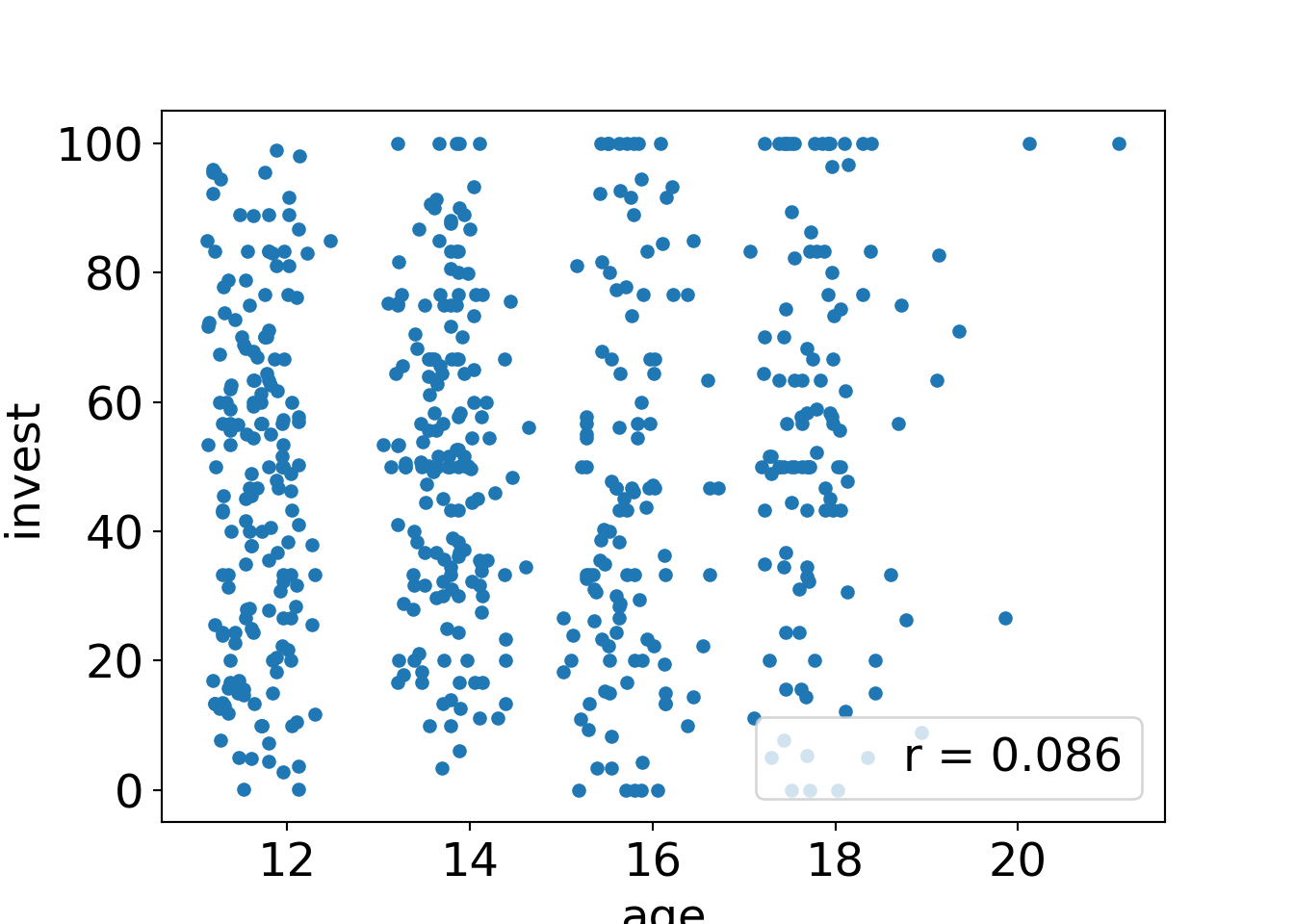
To illustrate testing the association of two quantitative variables, we consider a test of invest by age in the MLA data.

R

plot(invest ~ age, data = MLA)
legend("bottomright",
  paste("r =", round(cor(MLA[, c("invest", "age")])[2,1], 3)), bty = "n")

Python

r, p = stats.pearsonr(x=MLA["age"], y=MLA["invest"])

# Add Pearson correlation coefficient as label
MLA.plot.scatter(x="age", y="invest", label="r = {:.3f}".format(r))
plt.legend(markerscale=0)
plt.show();

The classical correlation measure for the (linear) correlation between two numeric variables is the Pearson product moment correlation.

R

The corresponding classical test for the null hypothesis of zero correlation is the default test in the cor.test() function in base R.

cor.test(~ age + invest, data = MLA, method = "pearson")

## 
##  Pearson's product-moment correlation
## 
## data:  age and invest
## t = 2.062, df = 568, p-value = 0.0397
## alternative hypothesis: true correlation is not equal to 0
## 95 percent confidence interval:
##  0.00408678 0.16712570
## sample estimates:
##       cor 
## 0.0861832

Note that the formula in the call above is not of the form y ~ x but rather ~ x + y. This is because R adopts the view that there is no dependent or explanatory variable but both variables enter equally. If in an analysis it is more natural to treat one of the variables as dependent (as is the case here), an analysis based on a linear regression (see next chapter) is probably preferable. However, note that the \(p\)-value from a simple linear regression is equivalent to that from the correlation test.

Python

print("cor = {:.3f}, p-value = {:.3f}".format(r, p))

## cor = 0.086, p-value = 0.040

Confidence interval for the Pearson’s correlation test:

# pearson's correlation test
r, p = stats.pearsonr(x=MLA["age"], y=MLA["invest"])

df = MLA["age"].size - 2 # degrees of freedom

se = np.sqrt((1-r**2)/df) # Standard error

alpha = 0.05 # Significant level (5%)

# Non-direction tests for computing t-critical value
t_critical = stats.t.ppf(1 - alpha / 2, df) # t_n-2;1-alpha/2

# Confidence interval
ci_low = r - t_critical*se
ci_hig = r + t_critical*se

print("{:.0f} percent confidence interval:".format(100*(1-alpha)))

## 95 percent confidence interval:

print("{:.5f}, {:.5f}".format(ci_low, ci_hig))

## 0.00408, 0.16829

To conduct the same test as a permutation test, we could either do so by hand (defining the test statistic as cor(y, x)) or by using the independence_test() function from coin as shown below:

R

independence_test(invest ~ age, data = MLA, distribution = approximate(10000))

## 
##  Approximative General Independence Test
## 
## data:  invest by age
## Z = 2.056, p-value = 0.0386
## alternative hypothesis: two.sided

Python

from r_functions import create
independence_test = create("coin.R", "independence_test")
res = independence_test(formula="invest ~ age", data="MLA.csv", distribution=10000)
print(res)

## {'method': 'Approximative General Independence Test', 'data': 'invest by age', 'statistic': 2.0558, 'pvalue': 0.0373, 'alternative': 'two.sided'}

The test statistic is scaled slightly differently but qualitatively both yield the same conclusions: There is a small positive correlation between investments and age which is just large enough to yield a \(p\)-value significant at 5% level.

Robust alternatives to the Pearson correlation are typically either the Spearman correlation or Kendall’s \(\tau\). The former is simply the Pearson correlation based on the rank-transformed observations. The latter counts pairs of observations that are concordant vs. discordant. Hence, both correlation measures capture monotonic (rather than linear) correlations.

R

In R, both are available as alternative methods in cor.test().

cor.test(~ age + invest, data = MLA, method = "spearman")

## Warning in cor.test.default(x = mf[[1L]], y = mf[[2L]], ...): Cannot compute exact
## p-value with ties

## 
##  Spearman's rank correlation rho
## 
## data:  age and invest
## S = 28915923, p-value = 0.132
## alternative hypothesis: true rho is not equal to 0
## sample estimates:
##       rho 
## 0.0631607

cor.test(~ age + invest, data = MLA, method = "kendall")

## 
##  Kendall's rank correlation tau
## 
## data:  age and invest
## z = 1.464, p-value = 0.143
## alternative hypothesis: true tau is not equal to 0
## sample estimates:
##       tau 
## 0.0413208

Note that the \(p\)-value computation of the Spearman test in cor.test() also employs a recursion algorithm similar to the Wilcoxon-Mann-Whitney test that only works exactly without ties. An alternative would be to employ independence_test() from coin, either by explicitly rank()-transforming both variables or by supplying rank as the xtrafo = and ytrafo =. Moreover, a dedicated spearman_test() interface is also available (which calls independence_test() internally).

independence_test(invest ~ age, data = MLA, distribution = approximate(10000),
  xtrafo = rank, ytrafo = rank)

## 
##  Approximative General Independence Test
## 
## data:  invest by age
## Z = 1.507, p-value = 0.131
## alternative hypothesis: two.sided

Python

rho, p = stats.spearmanr(MLA["age"], MLA["invest"])

print("rho = {:.3f}, p-value = {:.3f}".format(rho, p))

## rho = 0.063, p-value = 0.132

Spearman test with coin

spearman_test = create("coin.R", "spearman_test")
res = spearman_test(formula="invest ~ age", data="MLA.csv", distribution=10000)
print(res)

## {'method': 'Approximative Spearman Correlation Test', 'data': 'invest by age', 'statistic': 1.5066, 'pvalue': 0.134, 'alternative': 'true rho is not equal to 0'}

12.5.4 \(\chi^2\)-test in contingency tables

To illustrate testing the association of two qualitative variables, we consider the variables choice and gender in the Bookbinder’s Book Club (BBBClub) data. This had already been employed in the exploratory data analysis in Chapter 4, showing that the proportion of customers buying the advertised art book is considerably larger among women than among men.

R

tab <- xtabs(~ gender + choice, data = BBBClub)
tab

##         choice
## gender    no yes
##   female 273 183
##   male   627 217

prop.table(tab, 1)

##         choice
## gender         no      yes
##   female 0.598684 0.401316
##   male   0.742891 0.257109

Python

# Contingency table
tab = pd.crosstab(BBBClub['gender'], BBBClub['choice'])
print(tab)

## choice   no  yes
## gender          
## female  273  183
## male    627  217

# (Row) Normalized contingency table
tab_n = pd.crosstab(BBBClub['gender'], BBBClub['choice'], normalize= "index")
print(tab_n)

## choice      no     yes
## gender                
## female  0.5987  0.4013
## male    0.7429  0.2571

These conditional proportions are also displayed in a spine plot or mosaic plot:

R

A mosaic plot is produced by default in R:

plot(choice ~ gender, data = BBBClub)

Python

from statsmodels.graphics.mosaicplot import mosaic

grey_scale = lambda key: {'color': 'dimgrey' if 'yes' in key else 'lightgrey'} # Define a colo
mosaic(BBBClub, ["gender", "choice"], properties=grey_scale, gap=0.03);
plt.show()

The classical parametric test for formally testing the null hypothesis of independence between two qualitative variables is the \(\chi^2\)-test.

R

In R this is available as chisq.test() and in \(2 \times 2\) tables (fourfold tables) the default is to also apply a finite sample correction (Yates’ continuity correction):

chisq.test(tab)

## 
##  Pearson's Chi-squared test with Yates' continuity correction
## 
## data:  tab
## X-squared = 28.23, df = 1, p-value = 0.000000108

Python

Pearson’s Chi-squared test with Yates’ continuity correction

chi2, p, dof, ex = stats.chi2_contingency(tab)

print("X-squared = {:.0f}, df = {:.0f}, p-value = {:.0g}".format(chi2, dof, p))

## X-squared = 28, df = 1, p-value = 1e-07

Pearson’s \(\chi^2\)-test without Yates’ continuity correction:

R

chisq.test(tab, correct = FALSE)

## 
##  Pearson's Chi-squared test
## 
## data:  tab
## X-squared = 28.9, df = 1, p-value = 0.0000000762

Python

chi2, p, dof, ex = stats.chi2_contingency(tab, correction=False)

print("X-squared = {:.0f}, df = {:.0f}, p-value = {:.0g}".format(chi2, dof, p))

## X-squared = 29, df = 1, p-value = 8e-08

Both with or without the correction the test yields a highly-significant result confirming that the purchase probability depends on the gender.

The corresponding permutation test can be carried out with coin using the dedicated chisq_test() convenience interface to the generic independence_test() function.

R

library("coin")
chisq_test(tab, distribution = approximate(10000))

## 
##  Approximative Pearson Chi-Squared Test
## 
## data:  choice by gender (female, male)
## chi-squared = 28.9, p-value <0.0001

In addition to the interface based on the contingency "table" object tab, we could also call both functions for the \(\chi^2\)-test with the original variables. However, only chisq_test() from coin has a nice formula-based interface enabling chisq_test(choice ~ gender, data = BBBClub).

In contrast, the base chisq.test() function would need to be called as: chisq.test(BBBClub$gender, BBBClub$choice).

Python

chisq_test = create("coin.R", "chisq_test")
res = chisq_test(formula="choice ~ gender", data="BBBClub.csv", distribution=10000)
print(res)

## {'method': 'Approximative Pearson Chi-Squared Test', 'data': 'choice by gender (female, male)', 'statistic': 28.9014, 'pvalue': 0}

Note that the \(p\)-value is so small because none of the 10,000 permutations lead to a larger \(X^2\)-statistic than that observed on the original data. At first sight it might seem that the permutation \(p\)-value differs substantially from the asymptotic \(p\)-value above. However, with “only” 10,000 permutations it is not possible to obtain a \(p\)-value in the order of \(10^{-7}\). If we were to use a sufficiently large number of permutations, we would also obtain a \(p\)-value in a similar order of magnitude.

Finally, the exact \(p\)-value for assessing independence in contingency tables can be obtained directly without simulation (based on a hypergeometric distribution). Hence the corresponding test, known as Fisher’s exact test, is often applied instead of the \(\chi^2\)-test.

R

In R it is available as fisher.test():

fisher.test(tab)

## 
##  Fisher's Exact Test for Count Data
## 
## data:  tab
## p-value = 0.000000113
## alternative hypothesis: true odds ratio is not equal to 1
## 95 percent confidence interval:
##  0.402220 0.663346
## sample estimates:
## odds ratio 
##   0.516571

Python

from scipy.stats import fisher_exact

oddsr, p = fisher_exact(tab)

print("odds ratio = {:.3f}, p-value = {:.0g}".format(oddsr, p))

## odds ratio = 0.516, p-value = 1e-07