Chapter 11 Testing principles
Question: What is a general strategy for constructing a statistical test for a given problem?
In particular: What is a general strategy for constructing a statistical test for a 2-sample problem (including tests for location differences)?
11.1 Testing procedures
General strategy:
- Establish a null hypothesis and alternative.
- Compute a test statistic (based on the data) which captures deviations from the null hypothesis: It should be small under the null hypothesis but large or extreme under the alternative.
- Derive the distribution of the test statistic under the null hypothesis (based on assumptions about the theoretical distribution of the data) for computing critical values and \(p\)-values, respectively.
Example: Location difference in 2 samples.
- Null hypothesis: \(\mu_A = \mu_B\) vs. alternative \(\mu_A \neq \mu_B\).
- Test statistic: \((\overline y_A - \overline y_B)/\widehat{SD}\) (scaled difference of means).
- Null distribution: \(t\)-distribution or standard normal distribution (CLT).
In particular:
- Null hypothese/alternative: The null hypothesis that 2 samples come from the same distribution can be tested against many alternatives.
Example: Differences in mean or dispersion or skewness etc. - Test statistic: Various choices are possible.
Example: Difference of location measures: (trimmed) means, medians, etc.
Example: Ratio of dispersion measures.
Example: Difference of skewness coefficients.
- Null distribution: Only for some test statistics a CLT is available. And even if there is an asymptotic approximation, an exact test would be preferable.
Wanted: General strategy for obtaining the exact null distribution of a given test statistic.
Solution: Employ the permutation distribution.
11.2 Robust statistics
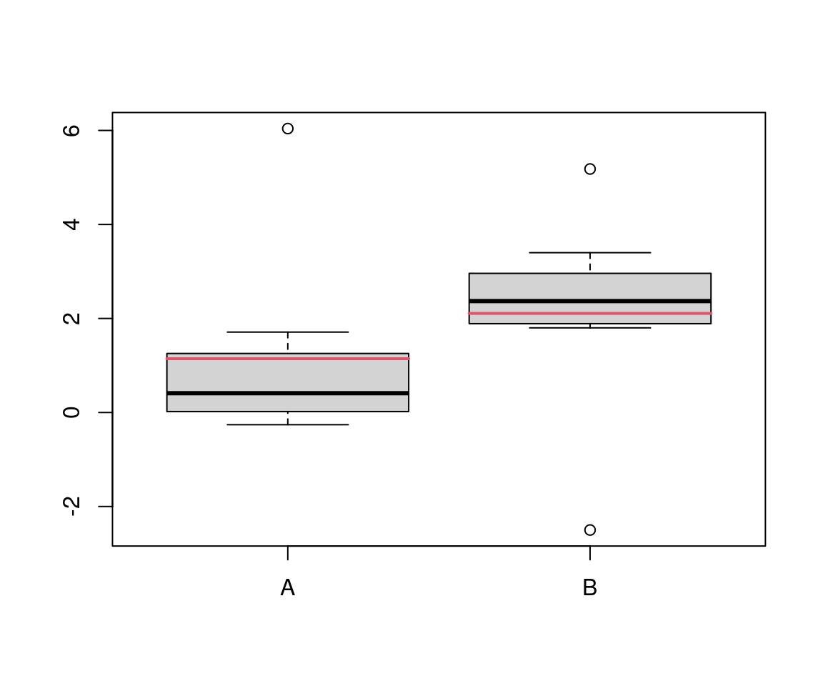
Problem: If the (empirical) distributions have “heavy” tails or if there are individual outliers, this can severely affect the empirical mean and it may become a poor location measure.
Example: Although the location in the center of the distribution differs clearly (\(Q_{A, 0.5} - Q_{B, 0.5} = -1.96\)), the corresponding means differ far less clearly (\(\overline y_A - \overline y_B = -0.96\)).
Solution: Employ a robust test statistic such as the median difference. \(p\)-values can be obtained from the permutation distribution (\(p = 0.047\)).
Comparison: Due to the outliers the \(t\)-test has little power (\(p = 0.412\)). Using the permutation distribution for the \(t\)-statistic yields almost equivalent results (\(p = 0.417\)).
Thus: The following two concepts should be distinguished.
- Permutation distribution: The null distribution (for computing critical values and \(p\)-values) can be obtained from the permutation principle even if no CLT is available or appropriate.
- Robust statistics: Test statistics on which outliers only have limited effects often have higher power if the data are very non-normal.
Note: Both concepts are often discussed jointly because robust tests are often conducted as permutation tests. However, both concepts can be applied separately.
11.3 \(t\)-test under different assumptions
Motivation: To introduce the general permutation principle for obtaining the null distribution, it is applied to the \(t\)-statistic \[ t \quad = \quad \frac{\overline y_A - \overline y_B}{\widehat{SD}} \] and compared to previous approaches based on different assumptions about the empirical data.
- Normal distribution: Asymptotic.
- \(t\)-distribution: Exact under normality.
- Permutation distribution: Exact given the observed data.
11.3.1 Asymptotic \(t\)-test
Previous assumptions: Two samples (of size \(n_A\) and \(n_B\)) from the random variables \(Y_A\) and \(Y_B\). No further assumptions about type and shape of the distributions of \(Y_A\) and \(Y_B\) are needed for the central limit theorem (CLT).
CLT: Under the null hypothesis the \(t\)-statistic is asymptotically standard normal.
Advantages: Few assumptions, very versatile.
Disadvantages: As \(n_A \rightarrow \infty\) and \(n_B \rightarrow \infty\) the approximation through the standard normal distribution keeps improving. However, it is unclear how well the approximation works in (small) finite samples.
11.3.2 \(t\)-test under normality
Moreover: If both random variables \(Y_A\) and \(Y_B\) are exactly normally distributed with equal variances \(\sigma_A^2 = \sigma_B^2\) and (under the null hypothesis) equal expectations \(\mu_A = \mu_B\), then the \(t\)-statistic is exactly \(t\)-distributed.
Advantages: Exact distribution.
Disadvantages: Only valid under normality. Whether this is actually the case, is typically unclear and hard to assess.
11.3.3 Practical remarks regarding \(t\)-tests
Remark: \(t\)-distribution and normal distribution already lead to very similar results for moderately large samples. Both work well when the samples “look normal”, i.e.,
- (approximately) symmetric,
- unimodal,
- few extreme observations or outliers.
But: If these properties do not hold, then the \(t\)-statistic itself is not well-suited. Furthermore, the significance level might be violated and/or the test might have low power under the alternative.
Transformation: For asymmetric samples, a log or square-root transformation can often help to transform the sample to approximately symmetric.
11.4 Permutation tests
11.4.1 Permutation distribution for the \(t\)-test
Idea:
- All computations are conditioned on the observed data.
- The corresponding empirical distribution is employed for obtaining the null distribution of the \(t\)-statistic.
Assumption: Under the null hypothesis the distributions of \(Y_A\) and \(Y_B\) are identical.
Thus: The assignment of labels \(A\) vs. \(B\) is completely random and without information. Labels can be permuted or re-randomized without changing the null distribution of the test statistic.
Name: Permutation principle leading to the permutation test.
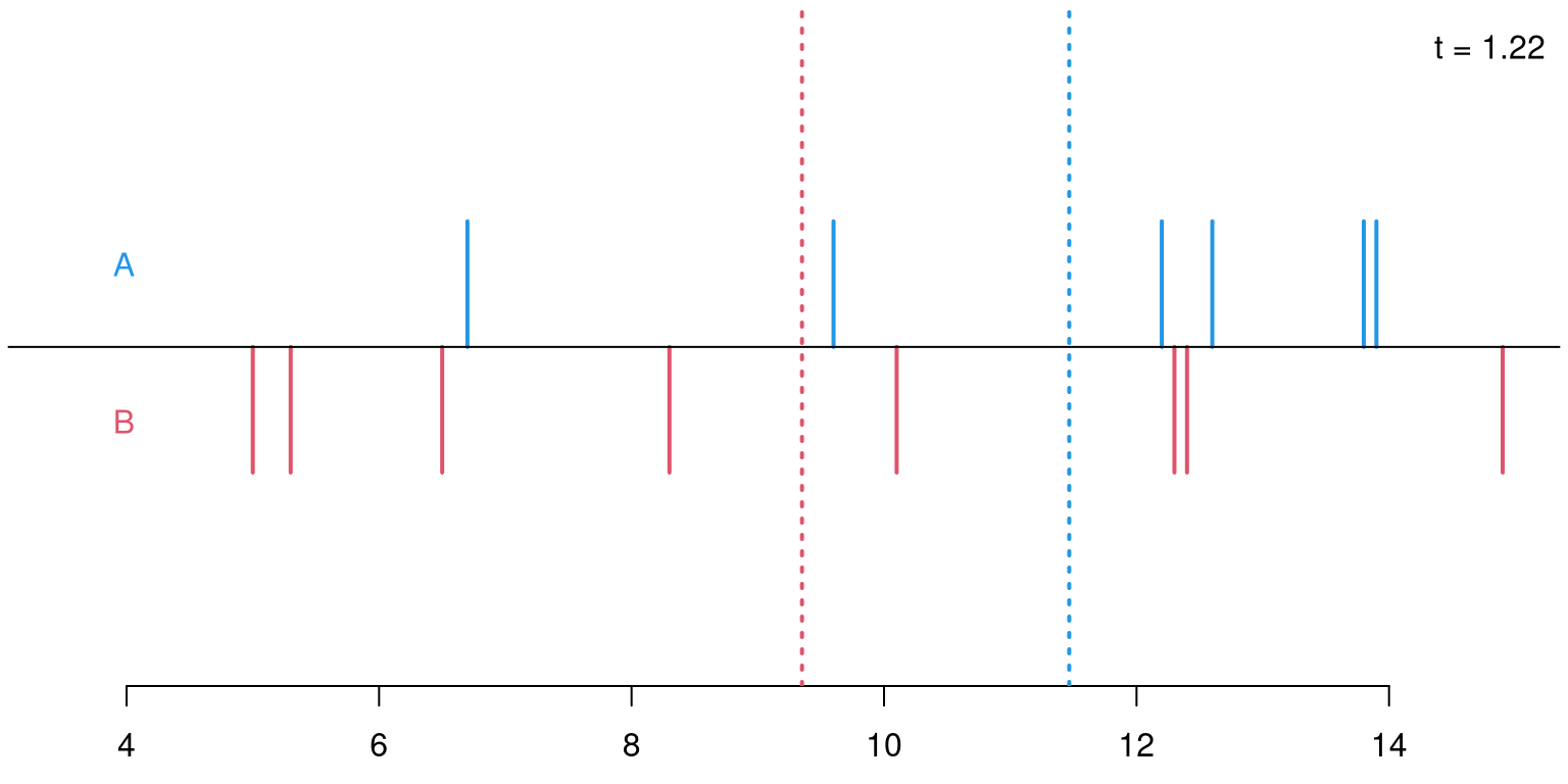
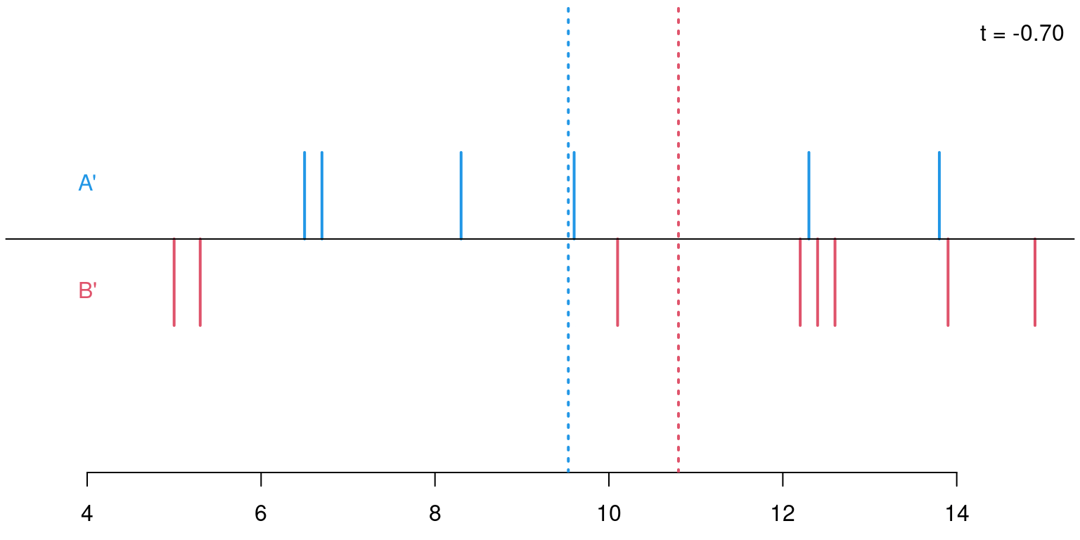
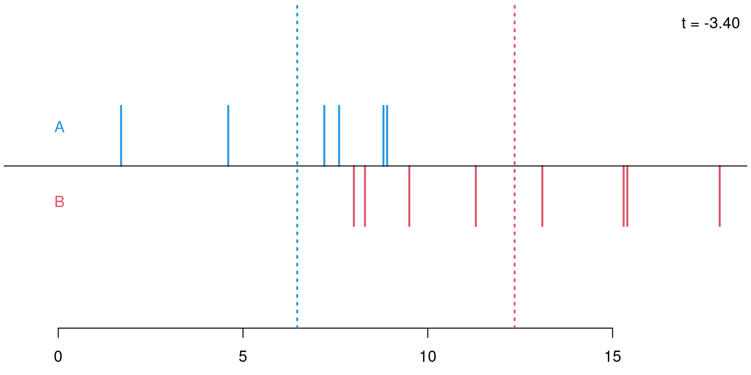
Permutations: For sample sizes of \(n_A = 6\) and \(n_B = 8\) there are \({ 14 \choose 6 } = 3003\) possible permutations of the response variable \(Y\) onto the explanatory variable \(X\) (i.e., its labels \(A\) and \(B\)).
Permutation distribution: For each of these possible permutations, evaluate the test statistic.
\(p\)-value: Proportion of statistics that deviate at least as much from \(0\) as the observed statistic. Here: \(p = 708/3003 = 0.236\). This \(p\)-value is virtually the same as the \(p\)-value based on the asymptotic normal distribution (\(p = 0.240\)) or \(t\)-distribution (\(p = 0.262\)), respectively.

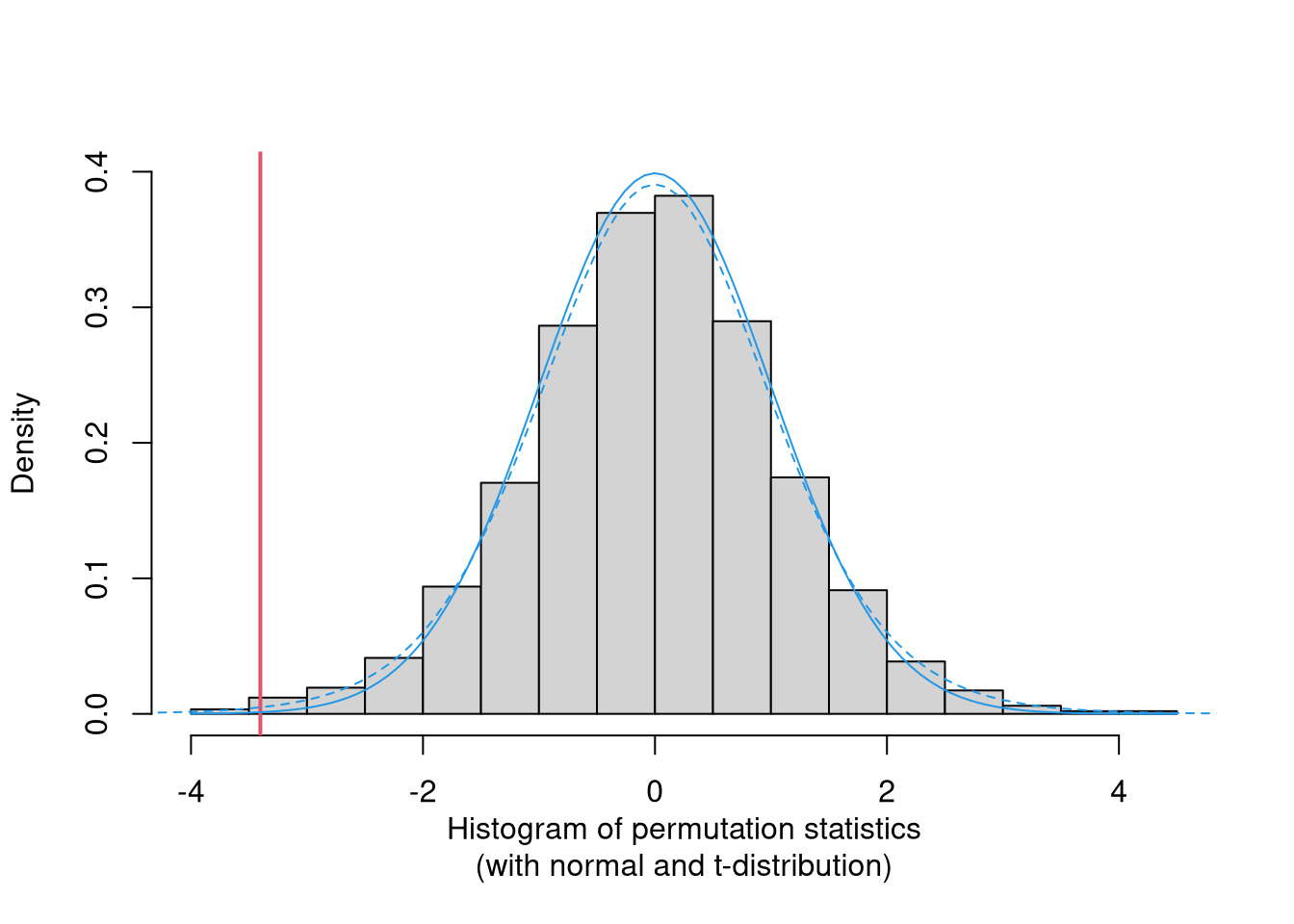
In general: The same principle can be applied to any statistic that contrasts two distributions: median difference, ratio of interquartile ranges, etc. In all cases the test statistic is evaluated on the observed data and all possible permutations to assess whether the observed statistic is extreme within the permutation distribution.
Advantage: Versatile, easy to interpret, exact distribution, independent of the underlying distribution of the data (even for finite \(n\)).
Disadvantage: Computationally intensive. The number of possible permutations grows exponentially with the number of observations.
Solution: Do not evaluate all possible evaluations but just a very large number, say 10,000 or similar.
In R: With package coin for “\(\underline{co}\)nditional \(\underline{in}\)ference”.
##
##  Approximative Two-Sample Fisher-Pitman Permutation Test
##
## data:  y by x (A, B)
## Z = 1.159, p-value = 0.253
## alternative hypothesis: true mu is not equal to 0##
## Approximative Two-Sample Fisher-Pitman Permutation Test
##
## data: y by x (A, B)
## Z = -2.474, p-value = 0.0078
## alternative hypothesis: true mu is not equal to 0Remark: Instead of the pooled estimator for \(\widehat{SD}\) this uses the 1-sample estimator.
11.5 Tutorial
11.5.1 Setup
Load the MLA data set. (The data set can be downloaded as MLA.csv or MLA.rda.)
R
##    invest      gender male     age treatment grade arrangement
## 1 70.0000 female/male  yes 11.7533      long   6-8        team
## 2 28.3333 female/male  yes 12.0866      long   6-8        team
## 3 50.0000 female/male  yes 11.7950      long   6-8        team
Python
11.5.2 Permutation tests with coin
An alternative approach for obtaining the null distribution for the \(t\)-test is the permutation principle. Thus, rather than assuming that the 2 samples come from normal distributions or relying on the central limit theorem, we can employ the permutation distribution conditional on the observed samples. The simple underlying idea is that under the null hypothesis it is random which observation falls into which of the 2 samples and may thus be permuted (i.e., re-randomized). First, we show how this can be done very conveniently using the coin package (for conditional inference) before implementing an entire permutation test from scratch in the next section.
The central workhorse function of the coin package is independence_test(y ~ x) which
conducts an independence test for any combination of y and x variable. The function does so
by employing transformations that are suitable for the scale of measurement of y and x, respectively.
Doing so the framework encompasses \(t\)-test, \(F\)-test, \(\chi^2\)-test, Wilcoxon-Mann-Whitney test, Spearman test and many others. Typical transformations include the identity, ranks, or dummy variables, among others. For all of the resulting independence test different null distributions can be used. The default is the asymptotic distribution which is either standard normal or the \(\chi^2\)-distribution. Alternatively, the null distribution can be approximated by sampling a (large) number of permutations. For certain tests - such as the Wilcoxon-Mann-Whitney test - the coin package also provides efficient algorithms to compute the permutation distribution exactly.
In addition to the core independence_test() function the coin package also comes with a number
of convenience interfaces that implement important special cases. For example, oneway_test()
is the counterpart to oneway.test() in base R or wilcox_test() is the counterpart to wilcox.test() and so on.
Here, we employ the function oneway_test() with 10,000 permutations for illustration. To make
results exactly reproducible a random seed is specified. The result is very similar to the asymptotic tests above.
R
The coin package can be easily installed from CRAN “as usual”, i.e., using the packages menu in RStudio or generally with the command install.packages("coin") and subsequently loaded in the current session with library("coin").
##
##  Approximative Two-Sample Fisher-Pitman Permutation Test
##
## data:  invest by treatment (long, short)
## Z = -1.268, p-value = 0.206
## alternative hypothesis: true mu is not equal to 0##
## Approximative Two-Sample Fisher-Pitman Permutation Test
##
## data: invest by arrangement (single, team)
## Z = -6.894, p-value <0.0001
## alternative hypothesis: true mu is not equal to 0Python
Unfortunately, there is no Python equivalent of the R package coin that implements several permutation tests.
Hence, we provide a Python interface to coin based on the Python package r_functions.
Setup
- Install R (https://discdown.org/rprogramming/installation.html).
- Install the R packages
coinandjsonliteviaRscript -e "install.packages(c('coin', 'jsonlite'), repos='https://cloud.r-project.org/', lib = .Library)"in your shell/prompt.- If you get the error
command not found, make sure to haveRsciptin yourPATH(https://stackoverflow.com/questions/38456144/rscript-command-not-found)
- If you get the error
- Install the Python package
r_functionsviapip install r-functions. - Download the coin.R file in the same folder of your notebook.
Usage
from r_functions import create

# create Python functions bound to R functions
oneway_test = create("coin.R", "oneway_test") # oneway ANOVA

###
#    oneway_test can be used as a Python function to compute oneway ANOVA using the permutation principle
#
#    :param formula: a string containing the R formula. For example:
#        formula ="invest ~ treatment" is the same as running anova_oneway with
#        data=MLA["invest"] and groups=MLA["treatment"]
#
#    :param data: a string containing the path to your dataset
#
#    :param distribution: string ("Asymptotic" - default, "Approximative", or "Exact") or integer (number of permutations)##
#
#    :returns: a dictionary with 'method', 'alternative', 'variables', 'statistic', and 'pvalue'
###

res = oneway_test(formula="invest ~ treatment", data="MLA.csv", distribution=10000)
print(res)
## {'method': 'Approximative Two-Sample Fisher-Pitman Permutation Test', 'data': 'invest by treatment (long, short)', 'statistic': -1.2681, 'pvalue': 0.2051, 'alternative': 'true mean is not equal to 0'}## {'method': 'Approximative Two-Sample Fisher-Pitman Permutation Test', 'data': 'invest by arrangement (single, team)', 'statistic': -6.8935, 'pvalue': 0, 'alternative': 'true mean is not equal to 0'}11.5.3 Permutation tests by hand
Instead of using the coin package it is also rather straightforward to conduct a permutation test by hand. For illustration, a permutation \(t\)-test is implemented from scratch below.
Three steps are used:
- The function
t_stat(y, x)computes the standard 2-sample \(t\)-statistic based on a numeric “response”yand binary explanatory factorx. - In addition to evaluating
t_stat(y, x)on the originalyandx, it is also evaluated on a large number of cases (e.g., 10,000) where the response is permuted:t_stat(sample(y), x). - From the resulting permutation distribution of the \(t\)-statistic \(p\)-values and critical values can be computed.
R
The function for step 1 employs tapply(y, x, function) for various functions to compute
mean, sd (standard deviation), and length (sample size) in each of the 2 samples.
These are then simply plugged into the equation for the \(t\)-statistic (using the pooled standard
deviation).
t_stat <- function(y, x)
{
  ## observed n, mean, sd
  n <- tapply(y, x, length)
  m <- tapply(y, x, mean)
  s <- tapply(y, x, sd)

  ## pooled variance and t-statistic
  pvar <- (n[1] + n[2]) / (n[1] * n[2]) *
    ((n[1] - 1) * s[1]^2 + (n[2] - 1) * s[2]^2) / (n[1] + n[2] - 2)
  tstat <- (m[1] - m[2]) / sqrt(pvar)

  return(tstat)
}
Python
def t_stat(y, x):
    data = pd.DataFrame({"y": y, "x": x})
    group_data = data.groupby("x")["y"]

    # observed n, mean, sd
    n = group_data.size().to_numpy()
    m = group_data.mean().to_numpy()
    s = group_data.std().to_numpy()

    # pooled variance and t-statistic
    pvar = (n[0] + n[1]) / (n[0] * n[1]) * \
    ((n[0] - 1) * s[0]**2 + (n[1] - 1) * s[1]**2) / (n[0] + n[1] - 2)
    tstat = (m[0] - m[1]) / np.sqrt(pvar)

    return tstat
In step 2 the function t_stat() is applied in nperm permutations, defaulting to nperm = 10000. As already stated above the permutation that breaks up the association of y and x (if any) can be easily carried out by the basic sample() function.
R
t_test <- function(y, x, nperm = 10000)
{
  ## observed statistic
  stat <- t_stat(y, x)

  ## statistic for permutations
  perm <- rep(0, nperm)
  for(i in 1:nperm) perm[i] <- t_stat(sample(y), x)

  ## return everything in a list
  ## (with class htest for automatic printing)
  rval <- list(
    statistic = c(t = stat),
    p.value = mean(abs(perm) >= abs(stat)),
    method = "Permutation t-test",
    permutations = perm
  )
  class(rval) <- "htest"
  return(rval)
}
Python
def t_test(y, x, nperm = 10000):
    # observed statistic
    stat = t_stat(y, x)

    ## statistic for permutations
    perm = np.zeros(nperm)
    for i in range(1, nperm):
        perm[i] = t_stat(np.random.permutation(y), x)

    # return everything in a dictionary
    tperm = {"statistic":[], "pvalue":[], "method":[], "permutations":[]}
    tperm["statistic"].append(stat)
    tperm["pvalue"].append(np.mean(np.abs(perm) >= np.abs(stat)))
    tperm["method"].append("Permutation t-test")
    tperm["permutations"].append(perm)

    return tperm
Finally, in step 3, the permutations are leveraged to compute a 2-sided \(p\)-value, which corresponds to the
proportion of more extreme permutations that are at least as high in absolute value as the originally-observed statistic.
The class "htest" is assigned to the list of results which has a print() method displaying
results of hypothesis tests in a standardized format.
Applying the t_test() function to the assessment of the treatment in the MLA experiment, yields
virtually the same result as the oneway.test() and oneway_test() functions above. (Replicating
the 1-sided t.test() result would require implementation of an alternative = argument in t_test() which was kept deliberately simple here.)
The resulting non-significant \(p\)-value is very close to the \(p\)-values from the \(t\)-distribution and asymptotic standard normal distribution:
The results for the arrangement test are:
Python
np.random.seed(403)
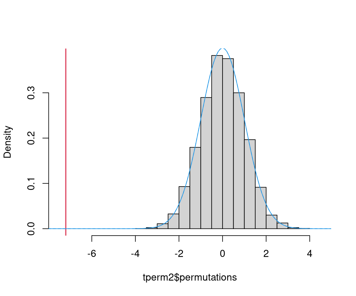
tperm2 = t_test(y=MLA["invest"], x=MLA["arrangement"], nperm=10000)
print(tperm2)## {'statistic': [np.float64(-7.194441325422449)], 'pvalue': [np.float64(0.0)], 'method': ['Permutation t-test'], 'permutations': [array([ 0. , 1.26605982, -0.46202587, ..., -1.30663328,
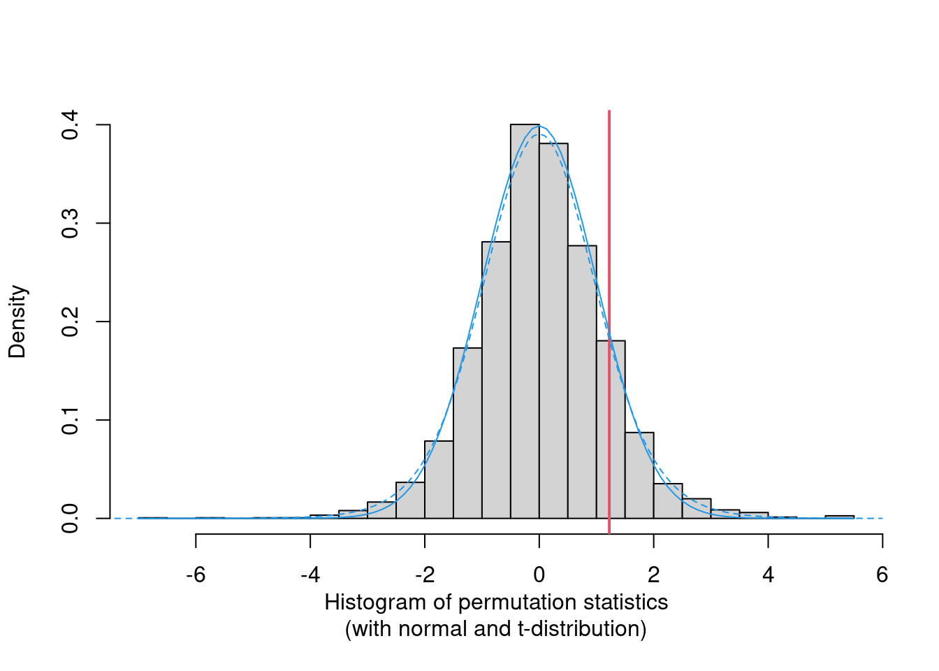
## -0.2600691 , 0.08704257])]}This shows that for a rather large sample with unimodal distribution that is not very skewed all three approaches for the null distribution (permutation distribution, normal approximation, \(t\)-distribution) yield very similar results and lead to qualitatively the same conclusions. Graphically, the three distributions can be compared in a histogram/density as shown below.
R
hist(tperm$permutations, freq = FALSE, col = "lightgray", main = "")
abline(v = tperm$statistic, col = 2, lwd = 2)
s <- seq(-8, 8, by = 0.1)
lines(s, dnorm(s), col = 4)
lines(s, dt(s, nrow(MLA) - 2), col = 4, lty = 2)
hist(tperm2$permutations, xlim = c(-7.5, 4.5), freq = FALSE, col = "lightgray", main = "")
abline(v = tperm2$statistic, col = 2, lwd = 2)
lines(s, dnorm(s), col = 4)
lines(s, dt(s, nrow(MLA) - 2), col = 4, lty = 2)
Python
fig, ax = plt.subplots(1, 2)

ax[0].hist(tperm["permutations"], density=True, color = 'lightgrey', edgecolor = 'black', bins=14)
ax[0].axvline(x=tperm["statistic"], color='r')
ax[0].set_xlabel('tperm - statistic')
ax[0].set_ylabel('Density')
density = stats.gaussian_kde(tperm["permutations"])
xs = np.linspace(-5,5,1000)
ax[0].plot(xs, density(xs))

ax[1].hist(tperm2["permutations"], density=True, color = 'lightgrey', edgecolor = 'black', bins=14)
ax[1].axvline(x=tperm2["statistic"], color='r')
ax[1].set_xlabel('tperm2 - statistic')
ax[1].set_ylabel('Density')
density = stats.gaussian_kde(tperm2["permutations"])
xs = np.linspace(-5,5,1000)
ax[1].plot(xs, density(xs))


fig.subplots_adjust(wspace=0.5)
plt.show()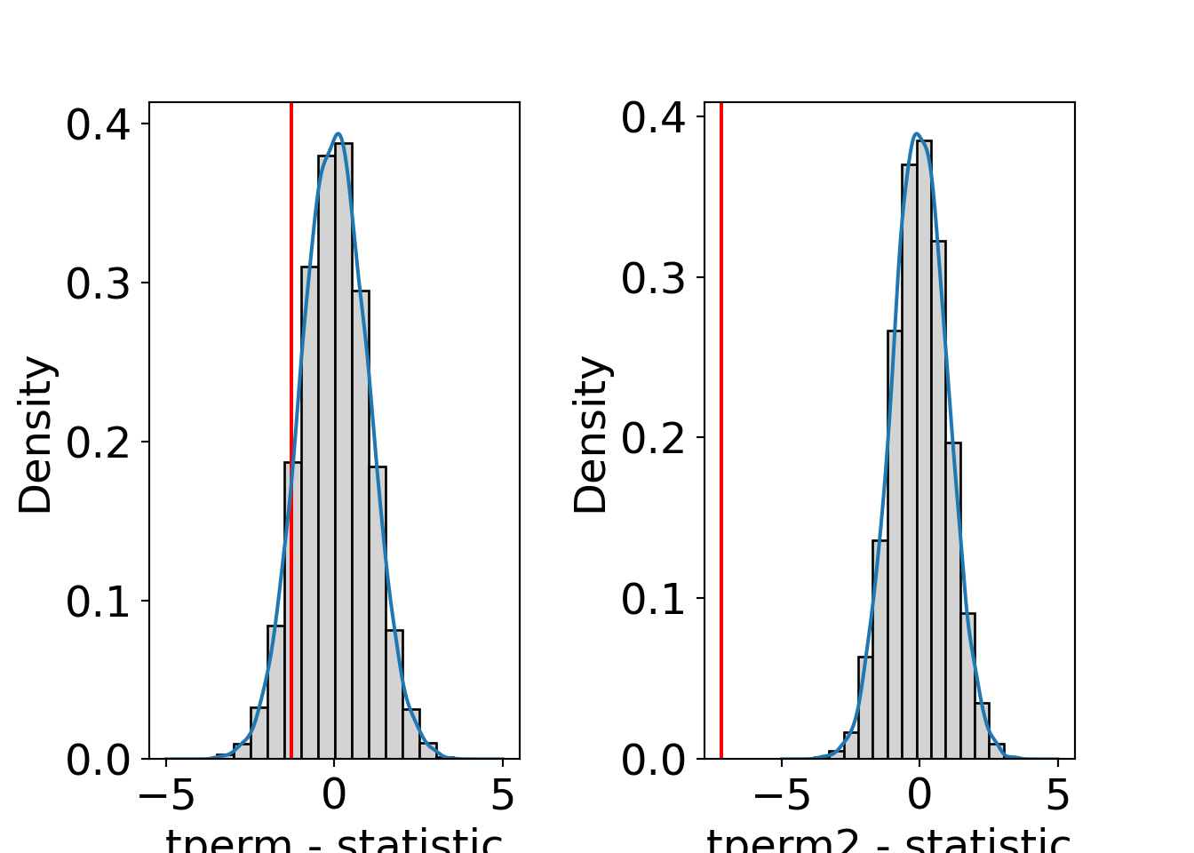
The permutation test is so appealing because it can be applied very easily and also works for other samples (small and/or multimodal and/or skewed). To obtain a powerful test it may be necessary, though, to employ a more robust test statistic than the \(t\)-statistic.
In terms of code there is not much in the t_test() function (except the method label) that
is specific to \(t\)-tests. Simply by re-defining the t_stat() function other test statistics
can also be used, e.g., a difference in means (without scaling by the standard deviation),
a difference in medians or trimmed means, etc. A slightly more elegant solution compared to
re-defining the t_stat() function would be to add an argument stat = t_stat that takes a
function for computing the test statistic.
Readers are encouraged to try out different versions of such a test by themselves. For example, they can explore different scalings for the \(t\)-statistic (pooled vs. 2-sample vs. no scaling) to see that this makes almost no difference for the permutation \(p\)-value.