Chapter 17 Logistic regression
17.1 Motivation
Previously: Linear regression model
\[\begin{eqnarray*} y_i & = & x_i^\top \beta ~+~ \varepsilon_i \\ \text{E}(y_i) ~=~ \mu_i & = & x_i^\top \beta \end{eqnarray*}\]
where the expectation \(\mu_i\) of a quantitative dependent variable \(y_i\) is modeled by a linear combination \(x_i^\top \beta\), using different explanatory variables (quantitative or qualitative with suitable numeric coding) and coefficient vector \(\beta\).
Linear predictor: \(x_i^\top \beta\) can assume values in the entire \(\mathbb{R}\).
Thus: Model equation is plausible if \(y_i\) can also assume values in the entire \(\mathbb{R}\). For non-negative quantitative variables (\(y_i > 0\)) this is sometimes achieved by using logarithms.
Problem: For many dependent variables this is not plausible, especially for binary variables and count data.
Binary variables: \(y_i \in \{0, 1\}\) signalling “failure” vs. “success”. \(\text{E}(y_i) = \mu_i \in (0, 1)\) is the success probability. Examples:
- Purchase decisions: Customer \(i\) buys/does not buy an advertised product.
Explanatory variables \(x_i\): Income, previous purchase history, age, … - Labor market participation: Woman \(i\) works/does not work.
Explanatory variables \(x_i\): Age, education, children, … - Credit risk: Person \(i\) pays/does not pay a credit back.
Explanatory variables \(x_i\): Income, credit history, maturity, occupation, age, marital status, …
Count data: \(y_i \in \{0, 1, 2, 3, \dots\}\) captures the number of events in some time window. \(\text{E}(y_i) = \mu_i \in (0, \infty)\). Examples:
- Purchase decisions: Number of products bought by customer \(i\).
Explanatory variables \(x_i\): Income, previous purchase history, age, … - Fertility: Number of children born by woman \(i\).
Explanatory variables \(x_i\): Education, ethnicity, siblings, … - Health economics: Number of doctor visits by person \(i\) in a year.
Explanatory variables \(x_i\): Age, gender, health, insurance, … - Leisure studies: Number of trips to a recreational resort by tourist \(i\).
Explanatory variables \(x_i\): Income, costs, costs of alternatives, …
Idea: Employ a link function \(g(\cdot)\) that maps the scale of the expectation \(\text{E}(y_i) = \mu_i\) to the scale of the linear predictor \(x_i^\top \beta\)
\[\begin{equation*} g(\mu_i) ~=~ x_i^\top \beta. \end{equation*}\]
Open questions:
- How to estimate the parameters \(\beta\)?
- How to carry out inference on \(\beta\) (hypothesis tests, confidence intervals)?
- What are natural choices for the link function \(g(\cdot)\)?
Trick: Fix the entire distribution of \(y_i\), not only its mean.
Example: In the linear regression model under assumptions (A1)–(A3) and (A6) the dependent variable is normally distributed as \(y_i \sim \mathcal{N}(\mu_i, \sigma^2)\).
Bernoulli distribution: Only possible distribution for a binary \(Y_i \in \{0, 1\}\) with
\[\begin{eqnarray*} \text{P}(Y_i = 1) & = & \mu_i, \\ \text{P}(Y_i = 0) & = & 1 - \mu_i. \end{eqnarray*}\]
Density function:
\[\begin{equation*} \text{P}(Y_i = y_i) ~=~ f(y_i; \mu_i) ~=~ \mu_i^{y_i} \cdot (1 - \mu_i)^{1 - y_i}. \end{equation*}\]
Moments: \(\text{E}(Y_i) = \mu_i\), \(\text{Var}(Y_i) = \mu_i \cdot (1 - \mu_i)\).
Remark: Special case of the binomial distribution (number of successes in \(N\) attempts) with \(N = 1\) attempt.
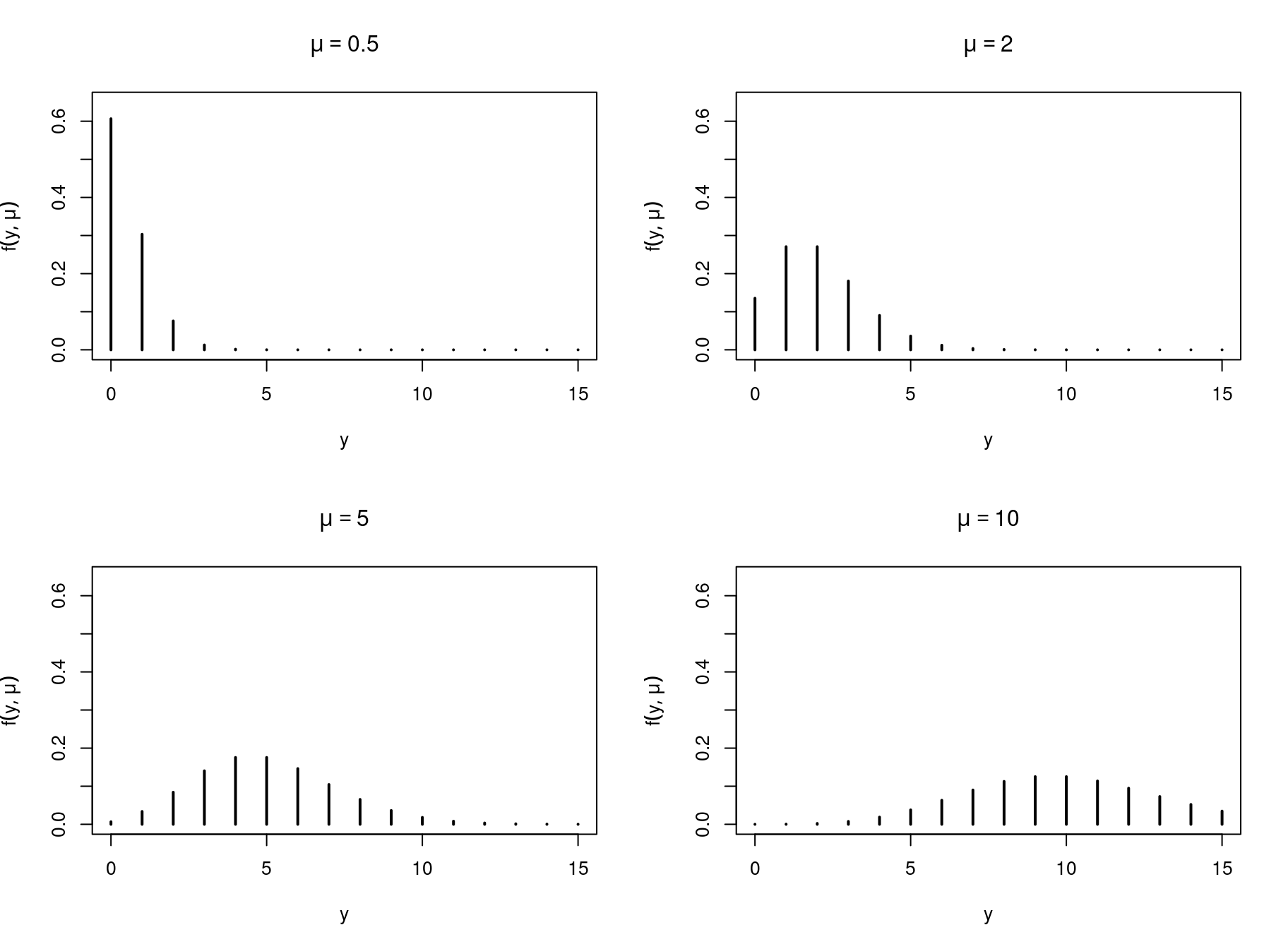
Poisson distribution: Basic distribution for count variable \(Y_i \in \{0, 1, 2, \dots\}\).
Density function:
\[\begin{equation*} \text{P}(Y_i = y_i) ~=~ f(y_i; \mu_i) ~=~ \frac{\mu_i^{y_i} \cdot \exp(-\mu_i)}{y_i!}. \end{equation*}\]
Moments: \(\text{E}(y_i) = \mu_i\), \(\text{Var}(y_i) = \mu_i\).
Remark: Both Bernoulli and Poisson distribution are per construction heteroscedastic. The variances vary along with the expectation. This was not the case for the normal variables with \(\text{Var}(y_i) = \sigma^2\).
Consequently: Ordinary least squares estimation cannot be efficient!
17.2 Maximum-likelihood estimation
Goal: Estimation of parameters in a model that has fixed the entire probability distribution of the dependent variable.
Starting point:
- \(n\) independent observations of a dependent variable: \(y_1, \dots, y_n\).
- Assumption of the corresponding probability distribution: \(f(y_i; \mu_i)\).
(Often, but not necessarily, \(\mu_i\) is the expectation. All ideas also work for distributions with multiple parameters.) - If explanatory variables are available: Link function \(\mu_i = h(x_i; \beta)\).
(Often, but not necessarily, based on a linear predictor: \(h(x_i; \beta) = \mu_i = g^{-1}(x_i^\top \beta)\).)
Idea:
- If the true parameter vector \(\beta\) were known, the full probability distribution could be computed. For example, the probability for observing a certain sequence of successes/failures \(y_1, \dots, y_n\) in a binary variable.
- When estimating the model, the data \(y_1, \dots, y_n\) has already been observed but the parameter \(\beta\) is unknown.
- Choose \(\beta\) such that the joint distribution/probability of observing the actual data is maximized.
Formally: The joint distribution, when considered as a function of the parameters for given data, is called likelihood.
\[\begin{equation*} L(\beta) ~=~ \prod_{i = 1}^n f(y_i; x_i, \beta). \end{equation*}\]
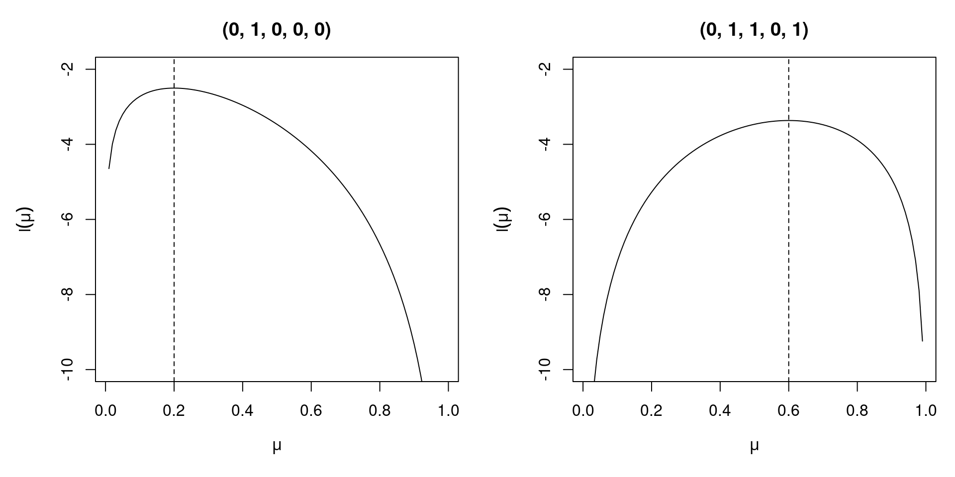
Alternatively: As sums are typically much nicer to handle both analytically and numerically, the likelihood is typically considered in logarithms.
\[\begin{equation*} \log L(\beta) ~=~ \ell(\beta) ~=~ \sum_{i = 1}^n \log f(y_i; x_i, \beta). \end{equation*}\]
Parameter estimation: The maximum-likelihood estimator (MLE) for \(\beta\) is then given by
\[\begin{equation*} \hat \beta ~=~ \underset{\beta}{\text{argmax}} ~ L(\beta) ~=~ \underset{\beta}{\text{argmax}} ~ \ell(\beta). \end{equation*}\]
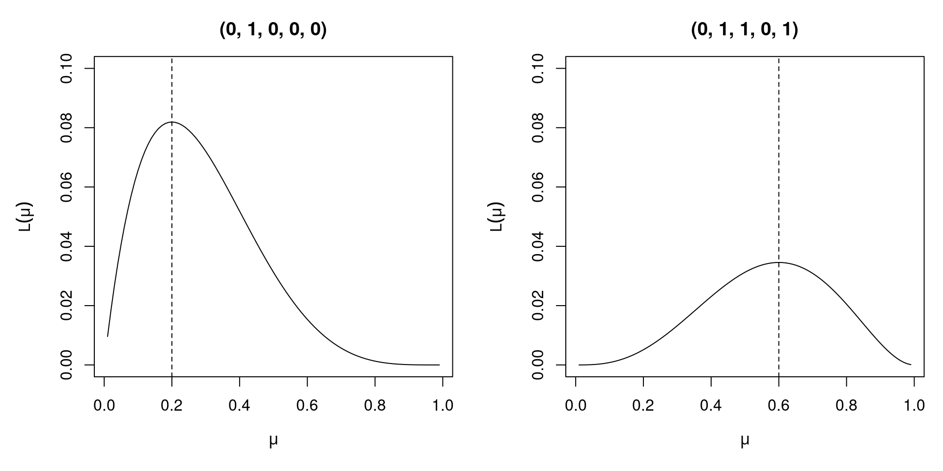
Illustration: 5 independent observations from a Bernoulli experiment with constant success probability \(\mu\) (i.e., without explanatory variables).
Likelihood: \(L(\mu)\) is the full joint probability
\[\begin{eqnarray*} L(\mu)& = & \text{P}(Y = y) ~=~ \prod_{i = 1}^5 \text{P}(Y_i = y_i) ~=~ \prod_{i = 1}^5 f(y_i; \mu) \\ & = & \prod_{i = 1}^5 \mu^{y_i} \cdot (1 - \mu)^{1 - y_i}. \end{eqnarray*}\]
Examples: Two different outcomes of the experiment.
- If \(y = (0, 1, 0, 0, 0)\) is observed, then \(L(\mu) = \mu \cdot (1 - \mu)^4\) with MLE \(\hat \mu = 0.2\).
- If \(y = (0, 1, 1, 0, 1)\) is observed, then \(L(\mu) = \mu^3 \cdot (1 - \mu)^2\) with MLE \(\hat \mu = 0.6\).
Properties: If the distribution is specified correctly and certain technical assumptions are valid, the MLE has certain optimality properties.
- Consistency: As the sample size \(n\) increases, \(\hat \beta\) tends to true parameter \(\beta\).
- Asymptotic normality: In large samples, \(\hat \beta\) has an approximate normal distribution.
- Efficiency: \(\hat \beta\) has a smaller asymptotic variance than other consistent uniformly asymptotically normal estimators.
Remark: Under assumptions (A1)–(A6) in the linear regression model the entire likelihood is also specified. In that situation OLS estimate and MLE coincide. (This is not the case for the other regression models considered in this chapter.)
Inference:
- Due to the asymptotic normality almost the same as in the linear model.
- \(t\)-tests for individual parameters, e.g., \(H_0: \beta_j = 0\), via
\[\begin{equation*} t ~=~ \frac{\hat \beta_j}{\widehat{\mathit{SD}(\hat \beta_j)}} \end{equation*}\]
\(F\)-tests for nested models. Similar to OLS but based on \(\ell(\beta)\) rather than \(\mathit{RSS}(\beta)\) as the objective function.
Information criteria:
\[\begin{eqnarray*} \mathsf{AIC}(\hat \beta) & = & -2 \cdot \ell(\hat \beta) ~+~ 2 \cdot k, \\ \mathsf{BIC}(\hat \beta) & = & -2 \cdot \ell(\hat \beta) ~+~ \log(n) \cdot k. \end{eqnarray*}\]
17.3 Binary response models
Open question: What are natural link functions for mapping the scale of the expectation \(\text{E}(y_i) = \mu_i\) to the scale of the linear predictor \(x_i^\top \beta\) (entire \(\mathbb{R}\)).
Initially: Consider the special case of a binary dependent variable \(y_i \in \{0, 1\}\) with success probability \(0 < \mu_i < 1\).
Even simpler: Consider only a single binary explanatory variable \(x_i \in \{0, 1\}\).
Example: choice (\(= y\)) explained by gender (\(= x\)) in the Bookbinder’s Book Club data BBBClub.
| Gender vs. choice | No | Yes |
|---|---|---|
| Women | 273 | 183 |
| Men | 627 | 217 |
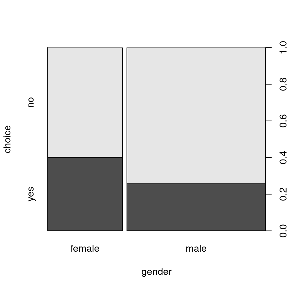
Excursion: Before tackling the link function, reconsider the exploratory analysis for this data.
Here: For investigating gender differences the conditional relative frequencies of choice given gender are more suitable.
| Gender vs. choice | No | Yes | Sum |
|---|---|---|---|
| Women | 0.599 | 0.401 | 1 |
| Men | 0.743 | 0.257 | 1 |
Odds: A more compact representation of these four relative frequencies is to employ odds instead of probabilities. The odds of an event are the ratio of the corresponding probability and the probability of the complementary event.
\[ \mathsf{Odds}(\mathsf{Choice} = \mathsf{Yes}) ~=~ \frac{\text{P}(\mathsf{Choice} = \mathsf{Yes})}{\text{P}(\mathsf{Choice} = \mathsf{No})} ~=~ \frac{\text{P}(\mathsf{Choice} = \mathsf{Yes})}{1 - \text{P}(\mathsf{Choice} = \mathsf{Yes})} \]
Here: Separately for women and men.
- Women: \(\mathsf{Odds}(\mathsf{Choice} = \mathsf{Yes}) = 0.401/0.599 = 0.67\), i.e., approx. \(2:3\).
- Men: \(\mathsf{Odds}(\mathsf{Choice} = \mathsf{Yes}) = 0.257/0.743 = 0.346\), i.e., approx. \(1:3\).
Odds ratio: \(0.346/0.67 = 0.516\), indicating that the odds of men purchasing the book are only half of women’s odds.
Note: The odds ratio can be easily computed directly from the table of absolute frequencies.
| Gender vs. choice | No | Yes |
|---|---|---|
| Women | 273 | 183 |
| Men | 627 | 217 |
\[ \mathsf{Odds} ~ \mathsf{Ratio} ~=~ \frac{273 \cdot 217}{627 \cdot 183} ~=~ 0.516 \]
In summary: The odds ratio can characterize the dependence of choice on gender in a single summary statistic.
Idea: Model the odds in a semi-logarithmic model. The coefficients then correspond to log-odds-ratios.
More formally: Employ the so-called logit function as the link function. \[ g(\mu) ~=~ \log \left( \frac{\mu}{1 - \mu} \right) \] This computes the log-odds. The corresponding regression model is also called logit model or logistic regression.
Model equation: Now fully specified.
\[\begin{equation*} \log \left( \frac{\mu_i}{1 - \mu_i} \right) ~=~ \log(\mathit{odds}_i) ~=~ x_i^\top \beta, \end{equation*}\]
where \(\beta\) can be estimated by maximum likelihood (while estimation via least squares is not straightforward!).
Interpretation: The logistic regression model captures log-odds conditional on the explanatory variables.
\[ \log \left( \frac{\text{P}(y_i = 1 ~|~ x_i)}{\text{P}(y_i = 0 ~|~ x_i)} \right) ~=~ x_i^\top \beta \]
Here: Women (\(x = 0\)) vs. men (\(x = 1\)).
\[\begin{eqnarray*} \frac{\text{P}(y = 1 ~|~ x = 1)}{\text{P}(y = 0 ~|~ x = 1)} & = & \exp(\beta_1 + \beta_2 \cdot 1) \\ \frac{\text{P}(y = 1 ~|~ x = 0)}{\text{P}(y = 0 ~|~ x = 0)} & = & \exp(\beta_1 + \beta_2 \cdot 0) \end{eqnarray*}\]
Odds ratio: \[\begin{eqnarray*} \frac{\exp(\beta_1 + \beta_2 \cdot 1)}{\exp(\beta_1 + \beta_2 \cdot 0)} & = & \frac{\exp(\beta_1 + \beta_2)}{\exp(\beta_1)} \\ & = & \exp(\beta_1 + \beta_2 - \beta_1) \\ & = & \exp(\beta_2) \end{eqnarray*}\]
Thus: Slope coefficients \(\beta\) in logistic regressions can be interpreted as changes in log-odds. Hence, \(\exp(\beta_j)\) is the odds ratio when \(x_j\) increases by one unit (and all other variables remain unchanged).
Here: The estimated coefficients are \(\displaystyle \beta = (-0.400, -0.661)^\top\) and hence the odds ratio is \(\exp(-0.661) = 0.516\). The odds of men purchasing the book are thus \(48.4\%\) lower than for women.
17.4 Tutorial
For illustrating generalized linear models (GLMs) with non-Gaussian dependent
variables the Bookbinder’s Book Club case study is employed. The BBBClub data set can be downloaded as BBBClub.csv or BBBClub.rda. For an exploratory
data analysis of the data see Chapter 4. The main
goal of the case study is to model the customers’ binary purchase choice of the
advertised book The Art History of Florence. A logistic regression model (or logit
model) is employed for this, selecting all relevant explanatory variables and their
pairwise interactions in a stepwise model selection.
17.4.1 Setup
Python
# Make sure that the required libraries are installed.
# Import libraries and classes:
import pandas as pd
import numpy as np
import matplotlib.pyplot as plt
import seaborn as sns
import statsmodels.api as sm
import statsmodels.formula.api as smf
from itertools import combinations
from statsmodels.graphics.mosaicplot import mosaic

from stepwise_selection import stepwise_selection, update_model

pd.set_option("display.precision", 4) # Set display precision to 4 digits in pandas and numpy.
# Load dataset
BBBClub = pd.read_csv("BBBClub.csv", index_col=False, header=0)
# Reorder categories for mosaic plots
BBBClub['choice'] = BBBClub['choice'].astype('category')
BBBClub['choice'].cat.reorder_categories(['yes', 'no'])## 0 yes
## 1 yes
## 2 yes
## 3 yes
## 4 yes
## ...
## 1295 no
## 1296 no
## 1297 no
## 1298 no
## 1299 no
## Name: choice, Length: 1300, dtype: category
## Categories (2, object): ['yes', 'no']17.4.2 Logistic regression
Question: Which variables in the Bookbinder’s Book Club data determine the decisions of the customers to purchase the advertised book about the art history of Florence?
Exploratory data analysis: At least visualization of all marginal relations between the
dependent variable choice and all potential explanatory variables.
R
plot(choice ~ art, data = BBBClub, breaks = c(-0.5, 0.5, 1.5, 2.5, 5.5))
plot(choice ~ gender, data = BBBClub)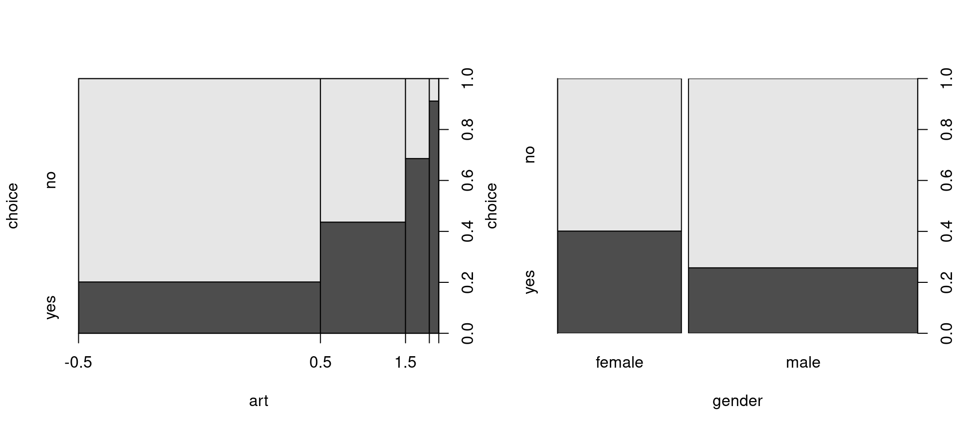
plot(choice ~ amount, data = BBBClub, breaks = fivenum(amount))
plot(choice ~ freq, data = BBBClub, breaks = fivenum(freq))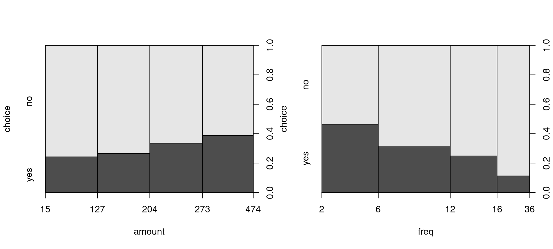
Python
BBBClub['art_bin'] = pd.cut(BBBClub['art'], [-0.5, 0.5, 1.5, 2.5, 5.5]) # Bin 'art' samples
grey_scale = lambda key: {'color': 'dimgrey' if 'yes' in key else 'lightgrey'} # Define a color map using lambda functionlambda key:
mosaic(data=BBBClub, index=['art_bin', 'choice'], properties=grey_scale, gap=0.05, statistic=True);
plt.show()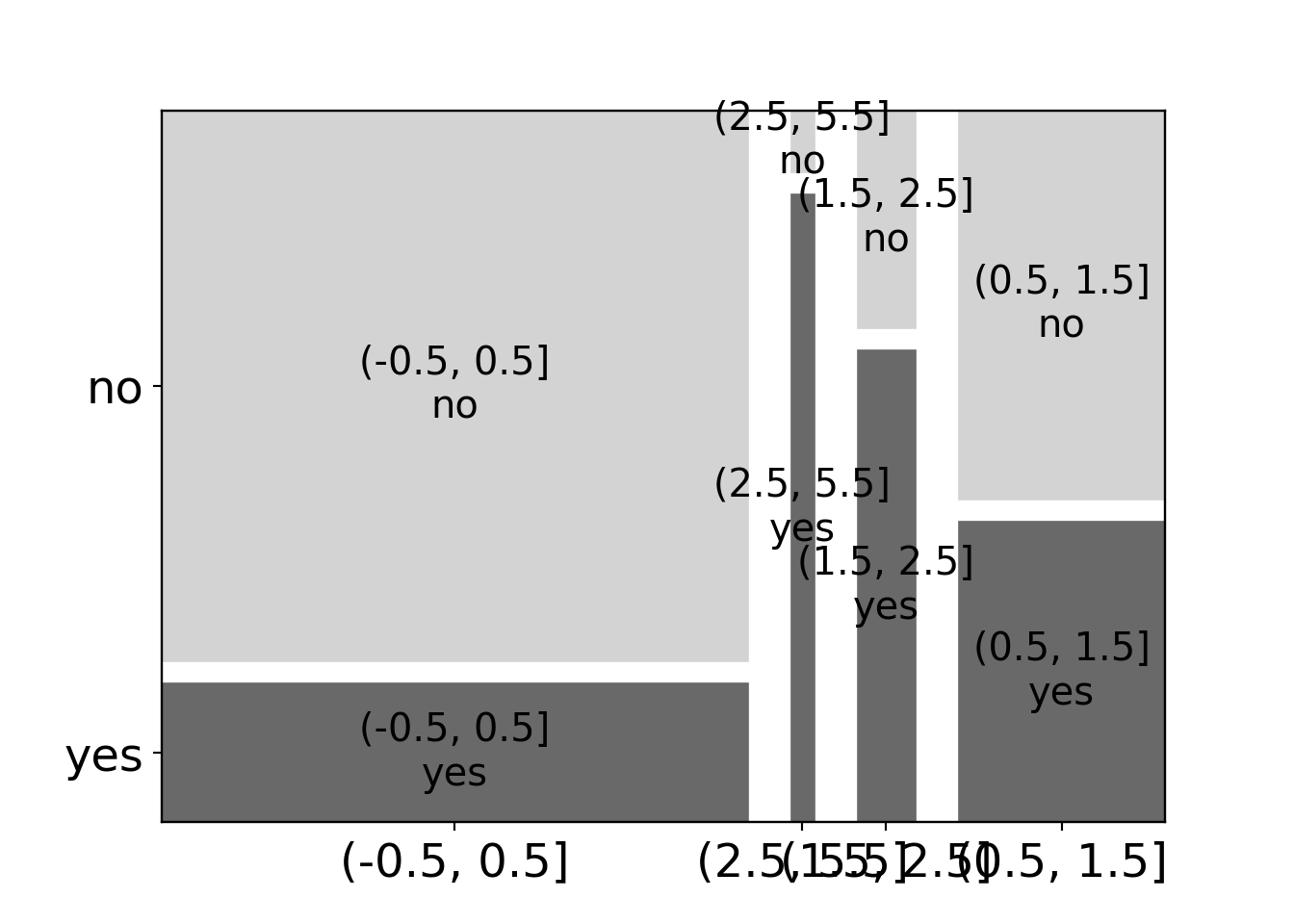
mosaic(data=BBBClub, index=['gender', 'choice'], properties=grey_scale, gap=0.02, statistic=True);
plt.show()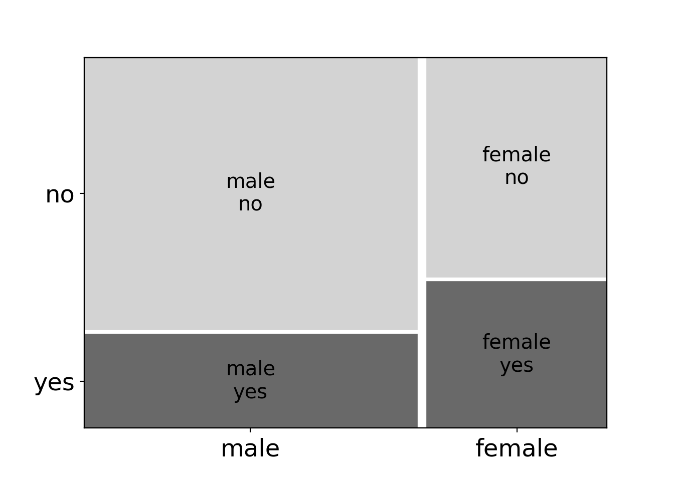
Five-numbers summary
We provide the fivenum() function to compute the five-number summary in {python}. We later use the five-number summary to define the braks in the mosaic plots.
def fivenum(data):
    """
    A function that computes the five-number summary.

    :param data: A column of 'pandas.DataFrame'
    :param column: The column of the DataFrame to use (string)

    :returns: The five numbers (list)
    """
    five_num = list()
    five_num.append(data.min()) # Min
    five_num.append(data.quantile(q=0.25)) # 1st Quantile
    five_num.append(data.quantile(q=0.5)) # Median
    five_num.append(data.quantile(q=0.75)) # 3st Quantile
    five_num.append(data.max()) # Max
return five_num## [np.int64(2), np.float64(6.0), np.float64(12.0), np.float64(16.0), np.int64(36)]BBBClub['amount_bin'] = pd.cut(BBBClub['amount'], fivenum(BBBClub['amount'])) # Bin 'amount' samples
mosaic(data=BBBClub, index=['amount_bin', 'choice'], properties=grey_scale, gap=0.02, statistic=True);
plt.show()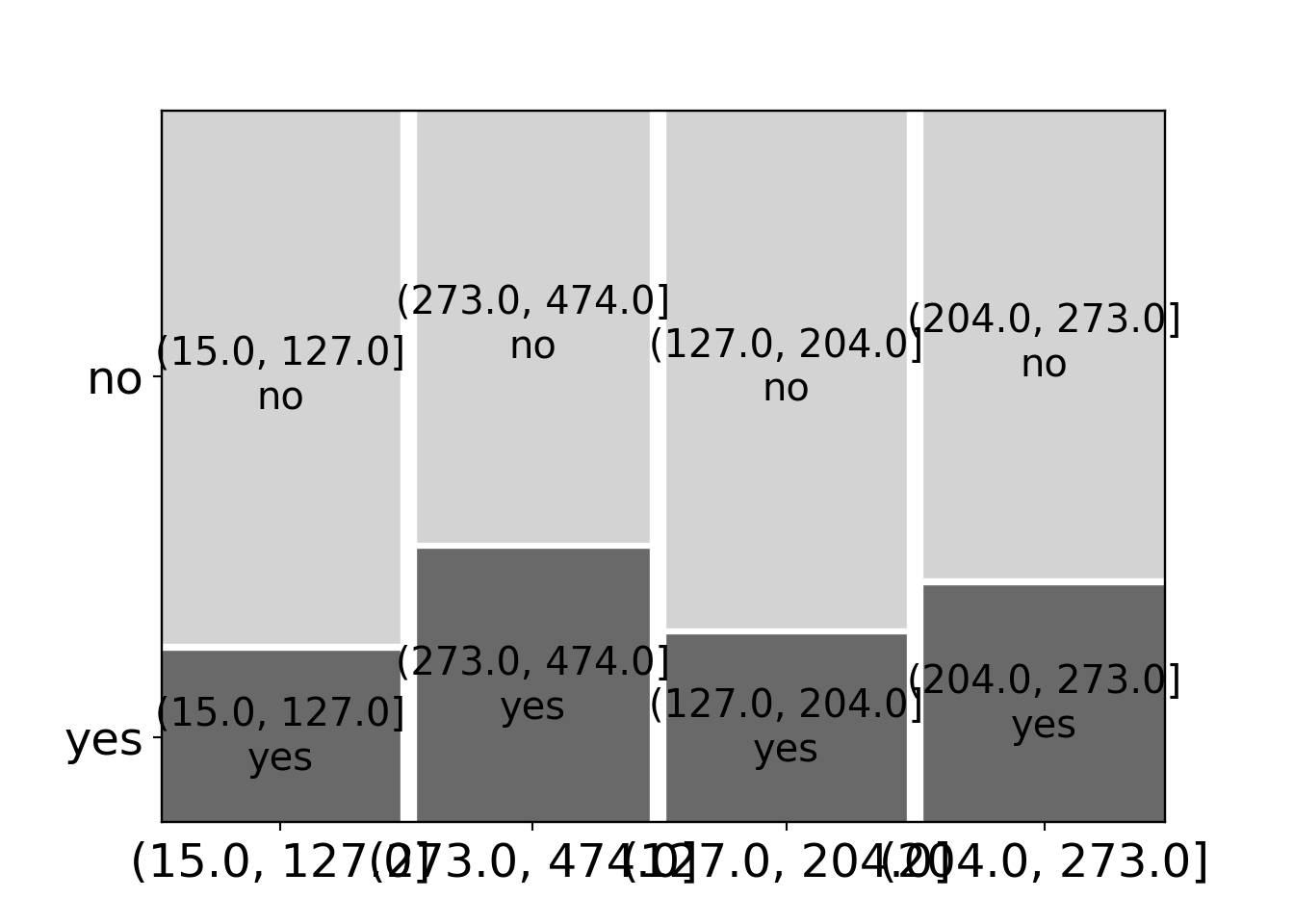
BBBClub['freq_bin'] = pd.cut(BBBClub['freq'], fivenum(BBBClub['freq'])) # Bin 'freq' samples
mosaic(data=BBBClub, index=['freq_bin', 'choice'], properties=grey_scale, gap=0.02, statistic=True);
plt.show()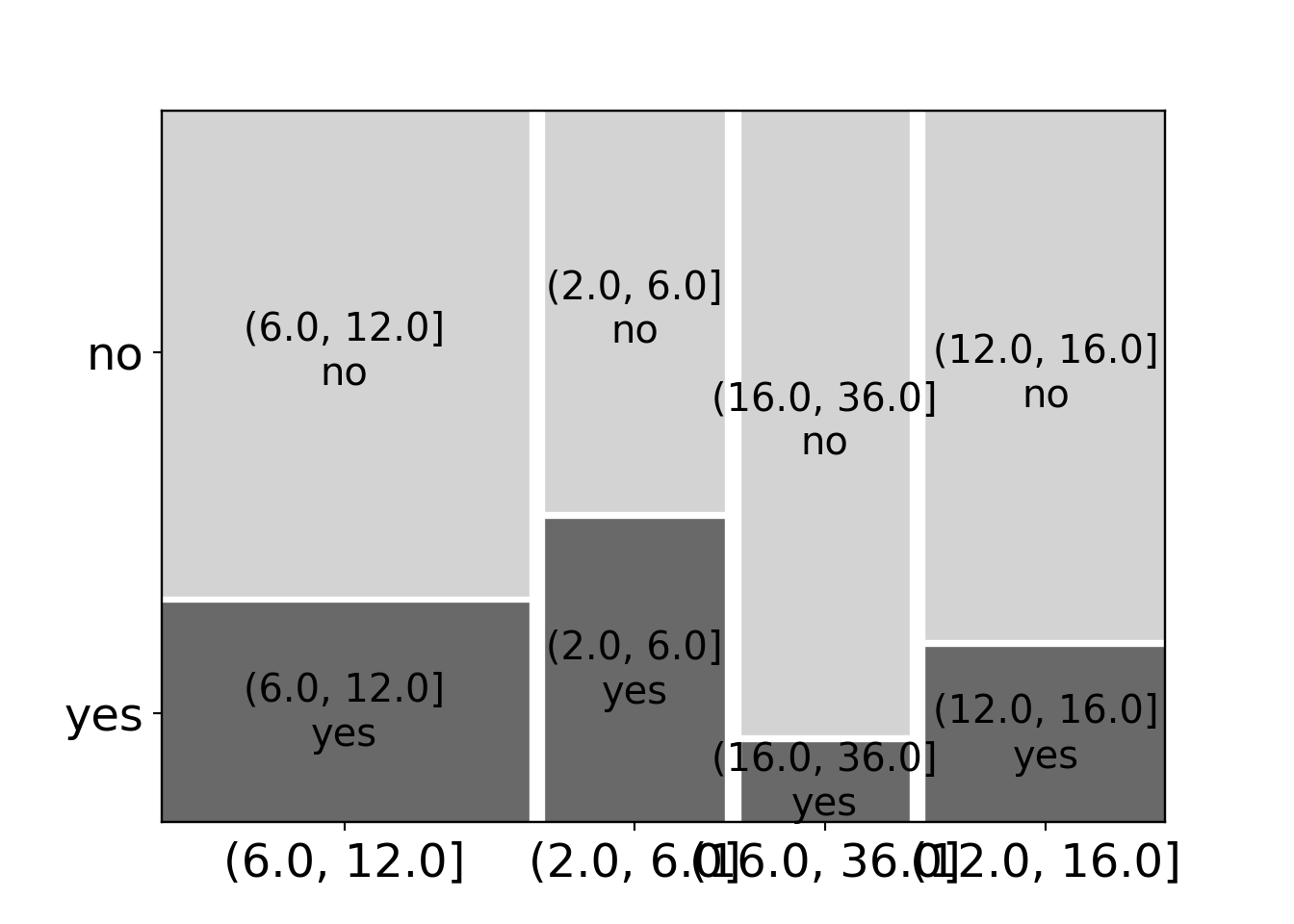
Logistic regression:
R
##
## Call:
## glm(formula = choice ~ gender, family = binomial(link = "logit"),
##     data = BBBClub)
##
## Coefficients:
##             Estimate Std. Error z value    Pr(>|z|)
## (Intercept)  -0.4000     0.0955   -4.19 0.000028308
## gendermale   -0.6611     0.1238   -5.34 0.000000093
##
## (Dispersion parameter for binomial family taken to be 1)
##
##     Null deviance: 1604.8  on 1299  degrees of freedom
## Residual deviance: 1576.4  on 1298  degrees of freedom
## AIC: 1580
##
## Number of Fisher Scoring iterations: 4
Python
# Statsmodels sorts the levels alphanumerically, therefore 'no' is '0' and 'yes' is '1'.
# Replace them
BBBClub1 = pd.read_csv("BBBClub.csv", index_col=False, header=0)
BBBClub1['choice'] = BBBClub1.choice.replace({"no": 0, "yes": 1})
## <string>:1: FutureWarning: Downcasting behavior in `replace` is deprecated and will be removed in a future version. To retain the old behavior, explicitly call `result.infer_objects(copy=False)`. To opt-in to the future behavior, set `pd.set_option('future.no_silent_downcasting', True)`m = smf.glm(formula="choice ~ gender", data=BBBClub1, family=sm.families.Binomial())
print(m.fit().summary())## Generalized Linear Model Regression Results
## ==============================================================================
## Dep. Variable: choice No. Observations: 1300
## Model: GLM Df Residuals: 1298
## Model Family: Binomial Df Model: 1
## Link Function: Logit Scale: 1.0000
## Method: IRLS Log-Likelihood: -788.22
## Date: Wed, 05 Mar 2025 Deviance: 1576.4
## Time: 14:23:50 Pearson chi2: 1.30e+03
## No. Iterations: 4 Pseudo R-squ. (CS): 0.02159
## Covariance Type: nonrobust
## ==================================================================================
## coef std err z P>|z| [0.025 0.975]
## ----------------------------------------------------------------------------------
## Intercept -0.4000 0.096 -4.187 0.000 -0.587 -0.213
## gender[T.male] -0.6611 0.124 -5.339 0.000 -0.904 -0.418
## ==================================================================================Model selection:
- Start with the binary GLM based on all main effects.
- Stepwise selection of additional effects, additionally considering all interactions with gender.
R
m1 <- glm(choice ~ gender + amount + freq + last + first +
  child + youth + cook + diy + art,
  data = BBBClub, family = binomial)
m2 <- step(m1, scope = list(lower = choice ~ 1,
  upper = choice ~ gender * (amount + freq + last + first + child + youth + cook + diy + art)
))
## Start: AIC=1244
## choice ~ gender + amount + freq + last + first + child + youth +
## cook + diy + art
##
## Df Deviance AIC
## - first 1 1222 1242
## + gender:diy 1 1219 1243
## <none> 1222 1244
## + gender:cook 1 1221 1245
## + gender:last 1 1221 1245
## + gender:freq 1 1222 1246
## + gender:youth 1 1222 1246
## + gender:amount 1 1222 1246
## + gender:art 1 1222 1246
## + gender:first 1 1222 1246
## + gender:child 1 1222 1246
## - amount 1 1227 1247
## - youth 1 1244 1264
## - art 1 1244 1264
## - freq 1 1245 1265
## - gender 1 1260 1280
## - last 1 1264 1284
## - diy 1 1267 1287
## - child 1 1275 1295
## - cook 1 1282 1302
##
## Step: AIC=1242
## choice ~ gender + amount + freq + last + child + youth + cook +
## diy + art
##
## Df Deviance AIC
## + gender:diy 1 1219 1241
## <none> 1222 1242
## + gender:cook 1 1221 1243
## + gender:last 1 1222 1244
## + gender:freq 1 1222 1244
## + gender:youth 1 1222 1244
## + gender:amount 1 1222 1244
## + first 1 1222 1244
## + gender:art 1 1222 1244
## + gender:child 1 1222 1244
## - amount 1 1227 1245
## - youth 1 1244 1262
## - art 1 1244 1262
## - gender 1 1260 1278
## - diy 1 1268 1286
## - last 1 1276 1294
## - child 1 1276 1294
## - cook 1 1284 1302
## - freq 1 1303 1321
##
## Step: AIC=1241
## choice ~ gender + amount + freq + last + child + youth + cook +
## diy + art + gender:diy
##
## Df Deviance AIC
## <none> 1219 1241
## - gender:diy 1 1222 1242
## + gender:art 1 1219 1243
## + gender:cook 1 1219 1243
## + gender:youth 1 1219 1243
## + gender:amount 1 1219 1243
## + gender:freq 1 1219 1243
## + first 1 1219 1243
## + gender:child 1 1219 1243
## + gender:last 1 1219 1243
## - amount 1 1224 1244
## - art 1 1241 1261
## - youth 1 1241 1261
## - child 1 1273 1293
## - last 1 1273 1293
## - cook 1 1280 1300
## - freq 1 1299 1319##
## Call:
## glm(formula = choice ~ gender + amount + freq + last + child +
## youth + cook + diy + art + gender:diy, family = binomial,
## data = BBBClub)
##
## Coefficients:
## Estimate Std. Error z value Pr(>|z|)
## (Intercept) -0.114909 0.224820 -0.51 0.609
## gendermale -0.750159 0.164340 -4.56 5.0e-06
## amount 0.001898 0.000848 2.24 0.025
## freq -0.090950 0.011240 -8.09 5.9e-16
## last 0.621587 0.088774 7.00 2.5e-12
## child -0.886666 0.128097 -6.92 4.5e-12
## youth -0.713144 0.158059 -4.51 6.4e-06
## cook -0.984553 0.132668 -7.42 1.2e-13
## diy -0.799288 0.190980 -4.19 2.8e-05
## art 0.643570 0.140189 4.59 4.4e-06
## gendermale:diy -0.390635 0.223032 -1.75 0.080
##
## (Dispersion parameter for binomial family taken to be 1)
##
## Null deviance: 1604.8 on 1299 degrees of freedom
## Residual deviance: 1219.3 on 1289 degrees of freedom
## AIC: 1241
##
## Number of Fisher Scoring iterations: 5Python
m1 = smf.glm("choice ~ gender + amount + freq + last + first + child + youth + cook + diy + art",
              data=BBBClub1, family=sm.families.Binomial())

m2 = stepwise_selection(m1, scope={"lower": "choice ~ 1",
                                   "upper": "choice ~ gender * \
                                   (amount + freq + last + first + child + youth + cook + diy + art)" })
## Step: aic= 1244.28170664869
## (' - first', np.float64(1242.4563874607377))
## (' + gender:diy', np.float64(1243.2021587144036))
## ('', np.float64(1244.28170664869))
## (' + gender:cook', np.float64(1244.7386195637364))
## (' + gender:last', np.float64(1245.4180444138876))
## (' + gender:freq', np.float64(1245.8334909527944))
## (' + gender:youth', np.float64(1245.9965551992254))
## (' + gender:amount', np.float64(1246.0800053602904))
## (' + gender:art', np.float64(1246.1030564641655))
## (' + gender:first', np.float64(1246.1211535163052))
## (' + gender:child', np.float64(1246.2429144134617))
## (' - amount', np.float64(1247.3724691203615))
## (' - youth', np.float64(1263.9019252907478))
## (' - art', np.float64(1264.1628685763926))
## (' - freq', np.float64(1265.233983599321))
## (' - gender', np.float64(1279.579018474739))
## (' - last', np.float64(1283.906790019139))
## (' - diy', np.float64(1287.277299021614))
## (' - child', np.float64(1295.2253142390737))
## (' - cook', np.float64(1302.0448594735312))
## Step: aic= 1242.4563874607377
## (' + gender:diy', np.float64(1241.3229759343394))
## ('', np.float64(1242.4563874607377))
## (' + gender:cook', np.float64(1242.8479640808898))
## (' + gender:last', np.float64(1243.5262512127929))
## (' + gender:freq', np.float64(1243.9904212734764))
## (' + gender:youth', np.float64(1244.1729922721283))
## (' + gender:amount', np.float64(1244.2721319492766))
## (' + first', np.float64(1244.28170664869))
## (' + gender:art', np.float64(1244.2989809132084))
## (' + gender:child', np.float64(1244.4003435165812))
## (' - amount', np.float64(1245.4882623384556))
## (' + gender:first', np.float64(1246.1211535163052))
## (' - youth', np.float64(1262.2135042747382))
## (' - art', np.float64(1262.2234576624105))
## (' - gender', np.float64(1277.8764533918043))
## (' - diy', np.float64(1285.8772592829264))
## (' - last', np.float64(1293.7179932156591))
## (' - child', np.float64(1294.0120687143067))
## (' - cook', np.float64(1301.7430275121023))
## (' - freq', np.float64(1321.0285711737772))
## Step: aic= 1241.3229759343394
## ('', np.float64(1241.3229759343394))
## (' - gender:diy', np.float64(1242.4563874607377))
## (' + gender:art', np.float64(1242.559112468882))
## (' + gender:cook', np.float64(1242.6179655841788))
## (' + gender:youth', np.float64(1242.6281574171792))
## (' + gender:amount', np.float64(1242.6568170981254))
## (' + gender:freq', np.float64(1242.7754693932452))
## (' + first', np.float64(1243.2021587144036))
## (' + gender:child', np.float64(1243.3016085653549))
## (' + gender:last', np.float64(1243.3223924901722))
## (' - amount', np.float64(1244.3681218608244))
## (' + gender:first', np.float64(1245.0139692305743))
## (' - art', np.float64(1260.959201617753))
## (' - youth', np.float64(1261.1995011277277))
## (' - child', np.float64(1292.7048286459658))
## (' - last', np.float64(1292.8715322066))
## (' - cook', np.float64(1300.266597856381))
## (' - freq', np.float64(1318.9387448274492))
## Result: aic= 1241.3229759343394
## choice ~ gender + amount + freq + last + child + youth + cook + diy + art + gender:diy## Generalized Linear Model Regression Results
## ==============================================================================
## Dep. Variable: choice No. Observations: 1300
## Model: GLM Df Residuals: 1289
## Model Family: Binomial Df Model: 10
## Link Function: Logit Scale: 1.0000
## Method: IRLS Log-Likelihood: -609.66
## Date: Wed, 05 Mar 2025 Deviance: 1219.3
## Time: 14:23:53 Pearson chi2: 1.28e+03
## No. Iterations: 5 Pseudo R-squ. (CS): 0.2566
## Covariance Type: nonrobust
## ======================================================================================
## coef std err z P>|z| [0.025 0.975]
## --------------------------------------------------------------------------------------
## Intercept -0.1149 0.225 -0.511 0.609 -0.556 0.326
## gender[T.male] -0.7502 0.164 -4.565 0.000 -1.072 -0.428
## amount 0.0019 0.001 2.239 0.025 0.000 0.004
## freq -0.0910 0.011 -8.092 0.000 -0.113 -0.069
## last 0.6216 0.089 7.002 0.000 0.448 0.796
## child -0.8867 0.128 -6.922 0.000 -1.138 -0.636
## youth -0.7131 0.158 -4.512 0.000 -1.023 -0.403
## cook -0.9846 0.133 -7.421 0.000 -1.245 -0.725
## diy -0.7993 0.191 -4.185 0.000 -1.174 -0.425
## gender[T.male]:diy -0.3906 0.223 -1.751 0.080 -0.828 0.046
## art 0.6436 0.140 4.591 0.000 0.369 0.918
## ======================================================================================Interpretation of the coefficients:
Python
## <string>:1: FutureWarning: Series.__getitem__ treating keys as positions is deprecated. In a future version, integer keys will always be treated as labels (consistent with DataFrame behavior). To access a value by position, use `ser.iloc[pos]`
## np.float64(1.209060589706953)## np.float64(1.8618814324299562)## np.float64(1.903262616669381)ANOVA GLM:
R
## Analysis of Deviance Table
##
## Model 1: choice ~ 1
## Model 2: choice ~ gender + amount + freq + last + child + youth + cook +
##     diy + art + gender:diy
##   Resid. Df Resid. Dev Df Deviance Pr(>Chi)
## 1      1299       1605
## 2 1289 1219 10 386 <2e-16## 'log Lik.' -609.7 (df=11)## 'log Lik.' -609.6 (df=11)Python
We provide the anova_glm() function to perform ANOVA with GLM (Binomial or Poisson) in {python}.
def anova_glm(m0, m1, test="Chisq"):
    """
    ANOVA for Generalized Linear Models (Binomial or Poisson).

    :param m0: a fitted GLM regression model from 'statsmodels' (Binomial or Poisson)
    :param m1: a fitted GLM regression model from 'statsmodels' (Binomial or Poisson)
    :param test: ANOVA test. Default "Chisq"

    :returns: The ANOVA table
    """
    # Check input are both Binomial or Poisson models
    binom_fam = sm.families.Binomial
    poiss_fam = sm.families.Poisson

    is_binom = isinstance(m0.family, binom_fam) and isinstance(m1.family, binom_fam)
    is_poiss = isinstance(m0.family, poiss_fam) and isinstance(m1.family, poiss_fam)

    if not (is_binom or is_poiss):
        raise TypeError("Models must be both 'Binomial' or 'Poisson'.")

    # Insert the ssr (sum of squared residuals) that is undefined for a binomial GLM
    m0.ssr = -2 * m0.llf
    m1.ssr = -2 * m1.llf

    # Return anova table
    return sm.stats.anova_lm(m0, m1, test=test)

m0 = update_model(m2, "choice ~ 1") # Well not really an update
m0_fit = m0.fit()

print(anova_glm(m0_fit, m2_fit, test="Chisq"))
## df_resid ssr df_diff ss_diff Chisq Pr(>Chisq)
## 0 1299 1604.8286 0.0 NaN 0.0 0.0
## 1 1289 1219.3230 10.0 385.5056 0.0 0.0