Chapter 15 Analysis of covariance
15.1 Introduction
Linear model: \(y_i = x_i^\top \beta + \varepsilon_i\) (with numeric dependent variable \(y\)) encompasses the following special cases.
- Linear regression: Sometimes denotes the case with quantitative explanatory variables \(x_i\). More often synonymous with linear model. Can be distinguished into simple and multiple linear regression.
- Analysis of variance: ANOVA. Analysis of nested linear models based on the corresponding variance decomposition.
- 1-way ANOVA: 1 qualitative explanatory variable (factor).
- 2-way ANOVA: 2 qualitative explanatory variables (factors).
- Analysis of covariance: ANCOVA. Mixed quantitative and qualitative explanatory variables, in particular when considering a mixed interaction effect.
Data:
##     invest arrangement   age
## 1    70.00        team 11.75
## 8    60.00        team 12.04
## 37   70.00        team 11.51
## 159  56.67        team 15.84
## 310  52.67      single 13.88
## 714  33.33      single 15.30
Univariate statistics:
##      invest      arrangement       age
##  Min.   :  0.0   single:385   Min.   :11.1
##  1st Qu.: 30.0   team  :185   1st Qu.:12.0
##  Median : 50.0                Median :13.9
##  Mean   : 50.4                Mean   :14.3
##  3rd Qu.: 70.0                3rd Qu.:15.9
##  Max.   :100.0                Max.   :21.1
Visualization:

Interaction model: Can be formulated equivalently via
invest ~ arrangement * age
invest ~ arrangement + age + arrangement:age
where the interaction effect arrangement:age results from the product of the corresponding main effects.
Model matrix:
##     (Intercept) arrangementteam   age arrangementteam:age
## 1             1               1 11.75               11.75
## 8             1               1 12.04               12.04
## 37            1               1 11.51               11.51
## 159           1               1 15.84               15.84
## 310           1               0 13.88                0.00
## 714           1               0 15.30                0.00
Model: Three actual regressors pertaining to two explanatory variables.
\[\begin{equation*} \mathit{invest}_i ~=~ \beta_1 ~+~ \beta_2 \cdot \mathit{team}_i ~+~ \beta_3 \cdot \mathit{age}_i ~+~ \beta_4 \cdot (\mathit{team}_i \cdot \mathit{age}_i) ~+~ \varepsilon_i. \end{equation*}\]
Distinction of cases: The indicator variable \(\mathit{team}_i\) can only assume two values, \(0\) for single players and \(1\) for teams.
\[\begin{eqnarray*} \mbox{If $\mathit{team}_i = 0$:} && \\ \mathit{invest}_i &=& \beta_1 ~+~ \beta_3 \cdot \mathit{age}_i ~+~ \varepsilon_i \\ \mbox{If $\mathit{team}_i = 1$:} && \\ \mathit{invest}_i &=& \beta_1 ~+~ \beta_2 ~+~ \beta_3 \cdot \mathit{age}_i ~+~ \beta_4 \cdot \mathit{age}_i ~+~ \varepsilon_i \\ &=& (\beta_1 + \beta_2) ~+~ (\beta_3 + \beta_4) \cdot \mathit{age}_i ~+~ \varepsilon_i \end{eqnarray*}\]
Interpretation:
- The interaction model corresponds to two separate simple linear regressions for both subsamples.
- The reference category has intercept \(\beta_1\) and slope \(\beta_3\).
- The other category has intercept \(\beta_1 + \beta_2\) and slope \(\beta_3 + \beta_4\).
- \(\beta_4\) is thus the difference in slopes. If \(\beta_4 = 0\), the slopes coincide, i.e., there is no interaction.
- \(\beta_2\) is thus the difference in intercepts. If \(\beta_2 = 0\), the intercepts coincide. Typically, this is only tested if \(\beta_4 = 0\) (or both, \(\beta_2\) and \(\beta_4\) are tested simultaneously).
15.2 Example
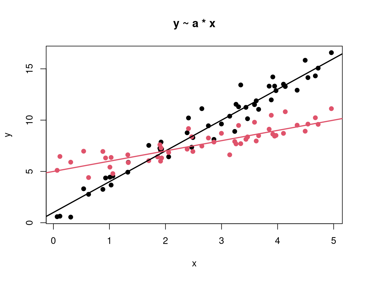
Example: Artificial data with quantitative dependent variable y and one qualitative explanatory variable a (black vs. red) and one quantitative explanatory variable x.
Known: Trivial model and models with only one main effect.
y ~ 1trivial model (1 mean)y ~ a1-way analysis of variance (2 means)y ~ xlinear regression (1 regression line)

New: Models with both explanatory variables.
y ~ a + x |
Main effect model (2 parallel regression lines) The lines have different intercepts according to a but the same slope with respect to x. |
y ~ a * x |
Interaction effect model (2 regression lines) The lines have both different intercepts and slopes with respect to x in the groups defined by a. Equivalent to: y ~ a + x + a:x. |

15.3 Application
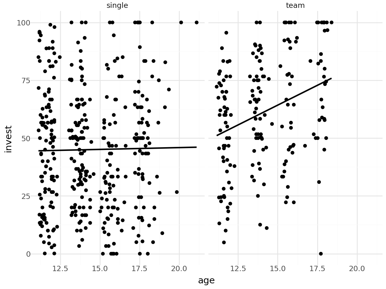
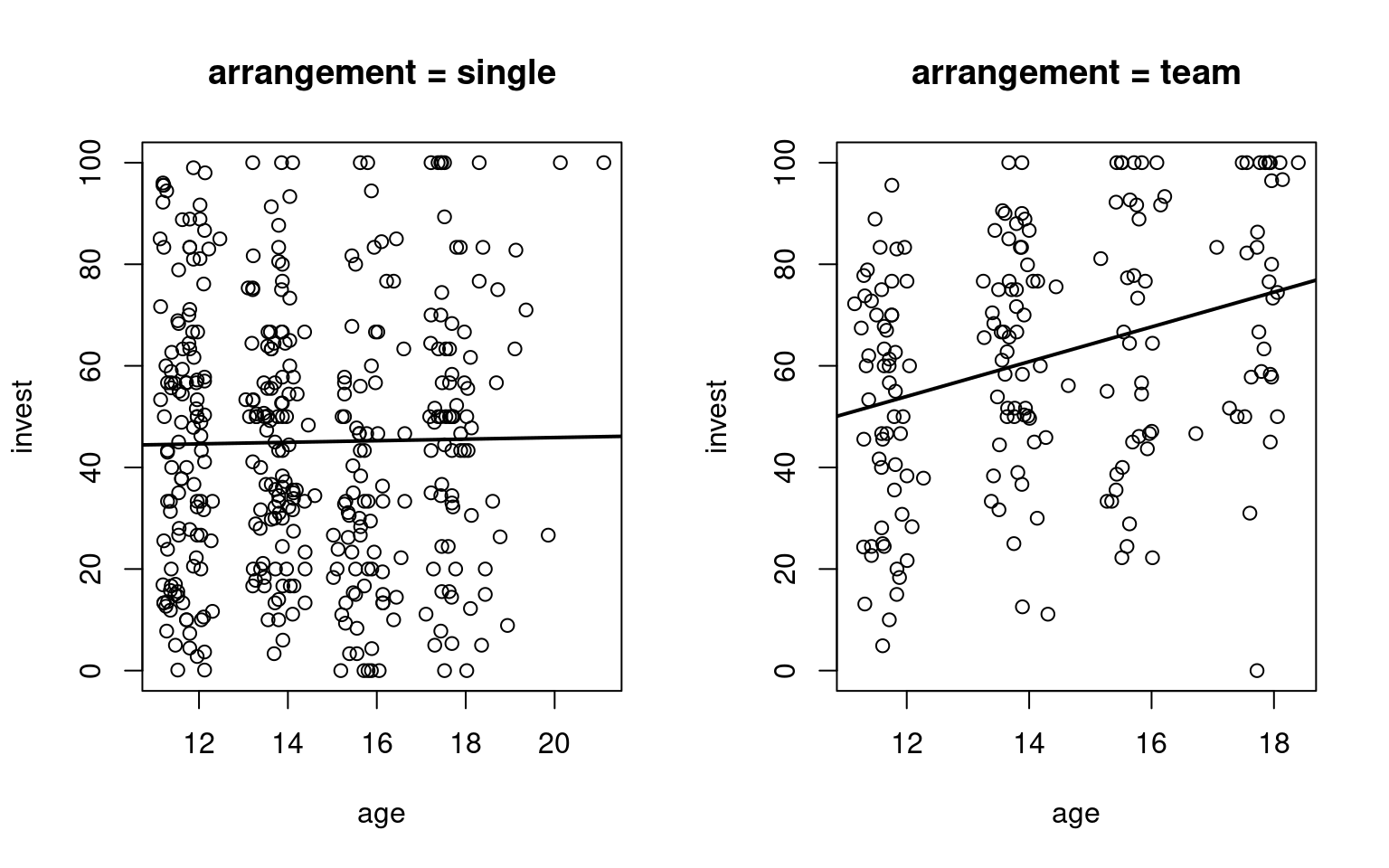
Example: Dependence of invest on arrangement and age of the players in the MLA data.
Model selection:
- The interaction effect is significant and thus the model cannot be simplified.
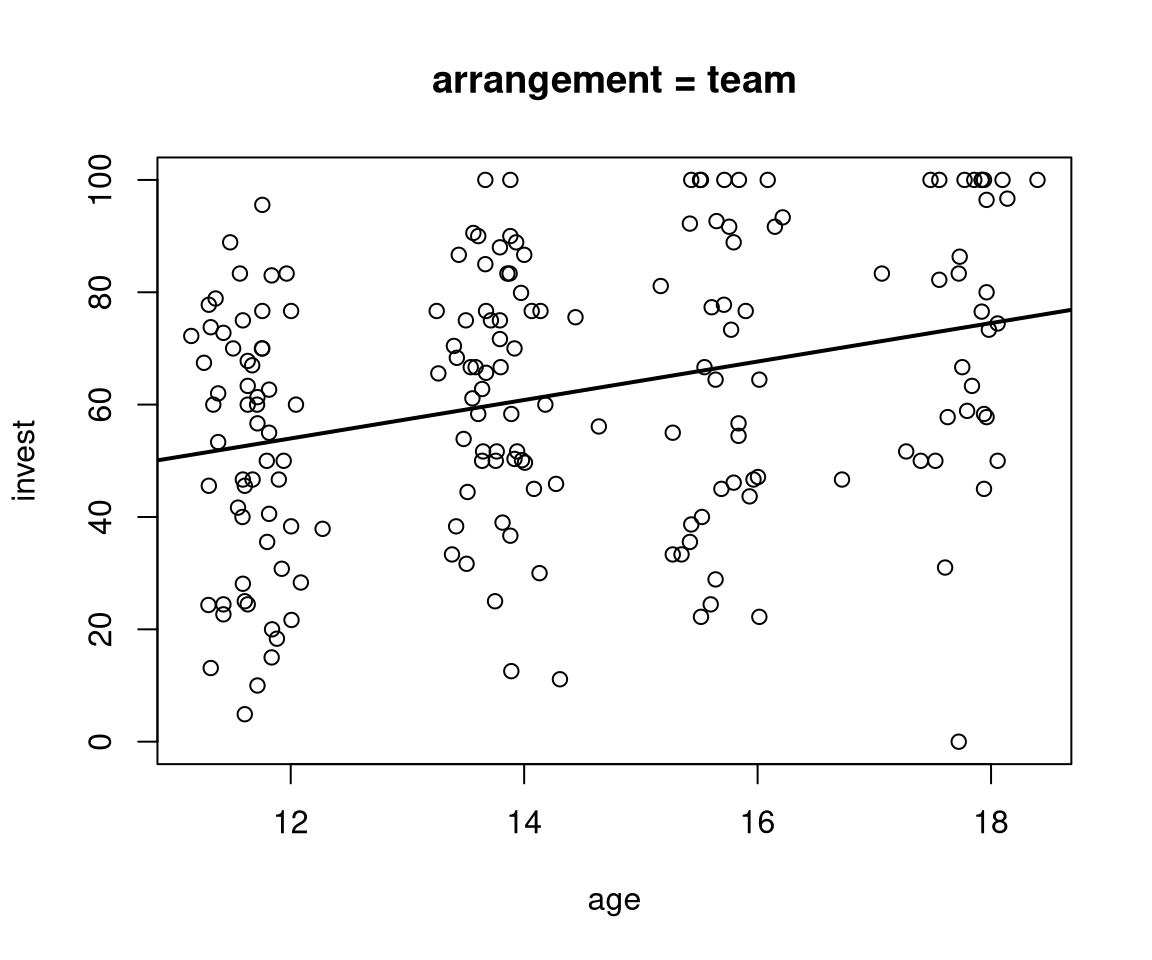
- The regression line with respect to age has different intercepts and slopes in the two arrangements.
- The age main effect in the reference group (single players) is not significant, indicating that in this group investments do not increase significantly with age.
- In the other group (teams) investments increase significantly (albeit only moderately) with age.

##
## Call:
## lm(formula = invest ~ arrangement * age, data = MLA)
##
## Residuals:
##    Min     1Q Median     3Q    Max
## -73.57 -20.81   1.21  18.44  55.17
##
## Coefficients:
##                     Estimate Std. Error t value   Pr(>|t|)
## (Intercept)           42.766      8.045    5.32 0.00000015
## arrangementteam      -29.846     14.584   -2.05     0.0412
## age                    0.156      0.552    0.28     0.7774
## arrangementteam:age    3.266      1.010    3.23     0.0013
##
## Residual standard error: 25.4 on 566 degrees of freedom
## Multiple R-squared:  0.109,  Adjusted R-squared:  0.105
## F-statistic: 23.2 on 3 and 566 DF,  p-value: 3.69e-14
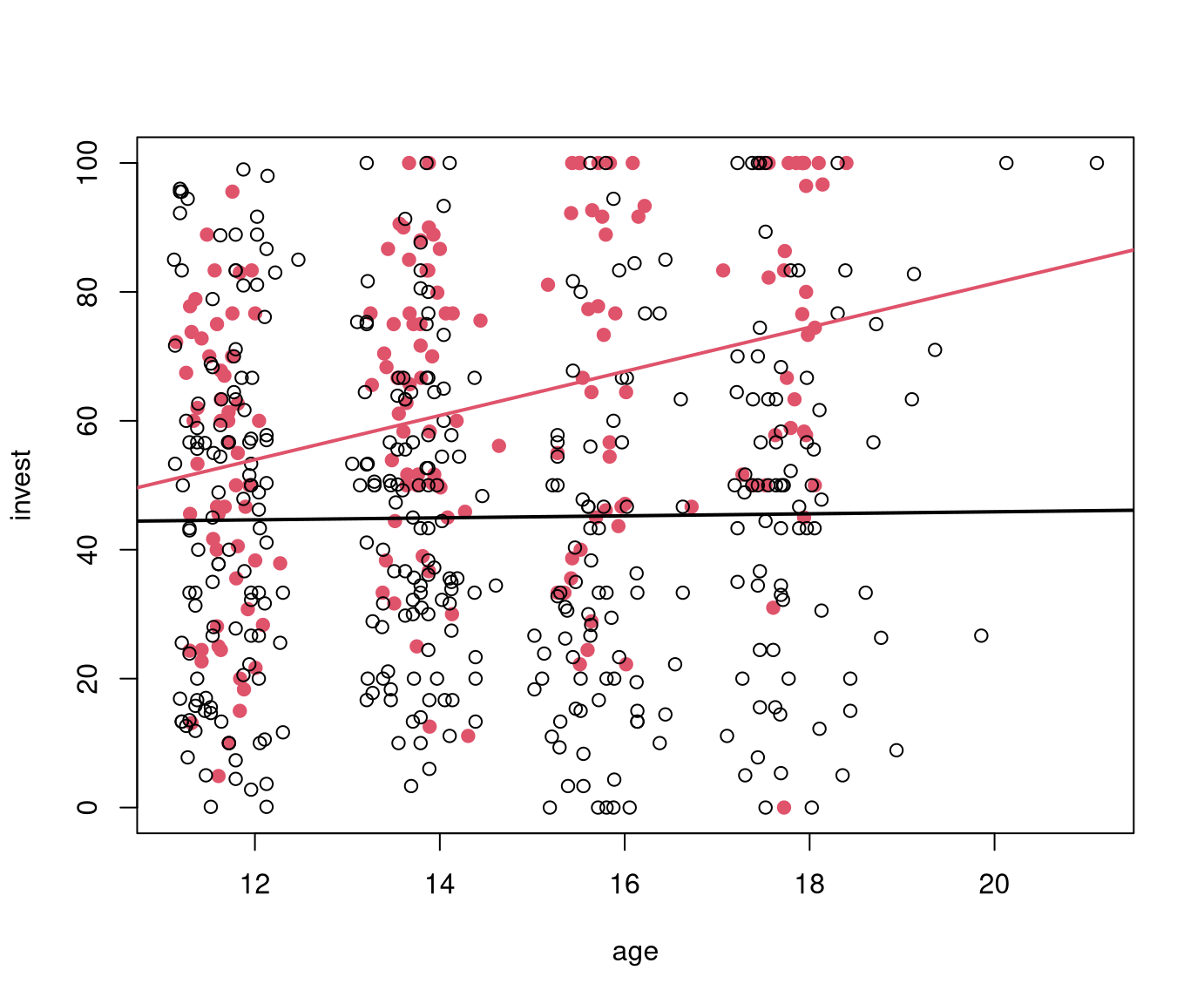
Interpretation:
- In the single arrangement the age slope is \(\hat \beta_3 = 0.156\).
- In the team arrangement the age slope is \(\hat \beta_3 + \hat \beta_4 = 3.422\).
- The intercepts (i.e., fitted values for age 0) are \(\hat \beta_1 = 42.766\) (single) and \(\hat \beta_1 + \hat \beta_2 = 12.92\) (team), respectively. These are not practically relevant, though.
- More interestingly, the regression lines take very similar values for a low age, e.g., age 11: \(44.483\) (single) vs. \(50.563\) (team). Thus, the team effect is much lower in lower age groups.
15.4 Tutorial
15.4.1 Setup
The myopic loss aversion (MLA) data (MLA.csv, MLA.rda) already analyzed in Chapters 13 and 14 are reconsidered. Here, the dependence of invested point percentages (invest) on all available explanatory variables and potential pairwise interaction is investigated, using analysis of variance for model selection.
R
##      invest       male          age       treatment     grade     arrangement
##  Min.   :  0.0   no :320   Min.   :11.1   long :285   6-8  :341   single:385
##  1st Qu.: 30.0   yes:250   1st Qu.:12.0   short:285   10-12:229   team  :185
##  Median : 50.0             Median :13.9
##  Mean   : 50.4             Mean   :14.3
##  3rd Qu.: 70.0             3rd Qu.:15.9
##  Max.   :100.0             Max.   :21.1
Python
# Make sure that the required libraries are installed.
# Import libraries and classes:
import pandas as pd
import numpy as np
import matplotlib.pyplot as plt
import seaborn as sns
import statsmodels.api as sm
import statsmodels.formula.api as smf
from itertools import combinations

pd.set_option("display.precision", 4) # Set display precision to 4 digits in pandas and numpy.## invest gender male age treatment grade arrangement
## count 570.0000 570 570 570.0000 570 570 570
## unique NaN 3 2 NaN 2 2 2
## top NaN female no NaN long 6-8 single
## freq NaN 320 320 NaN 285 341 385
## mean 50.3784 NaN NaN 14.3331 NaN NaN NaN
## std 26.8094 NaN NaN 2.3029 NaN NaN NaN
## min 0.0000 NaN NaN 11.1256 NaN NaN NaN
## 25% 30.0000 NaN NaN 11.9782 NaN NaN NaN
## 50% 50.0000 NaN NaN 13.8756 NaN NaN NaN
## 75% 70.0000 NaN NaN 15.9397 NaN NaN NaN
## max 100.0000 NaN NaN 21.1064 NaN NaN NaN## invest gender male age treatment grade arrangement
## 0 70.0000 female/male yes 11.7533 long 6-8 team
## 1 28.3333 female/male yes 12.0866 long 6-8 team
## 2 50.0000 female/male yes 11.7950 long 6-8 team
## 3 50.0000 male yes 13.7566 long 6-8 team
## 4 24.3333 female/male yes 11.2950 long 6-8 team15.4.2 Analysis of covariance
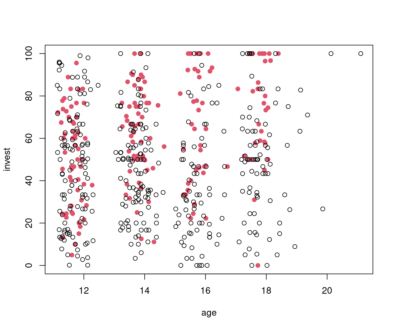
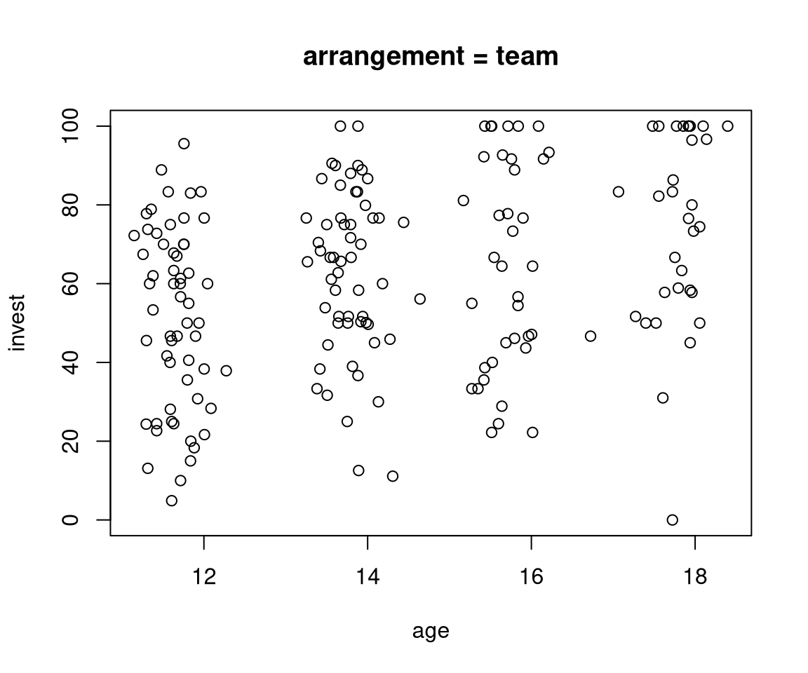
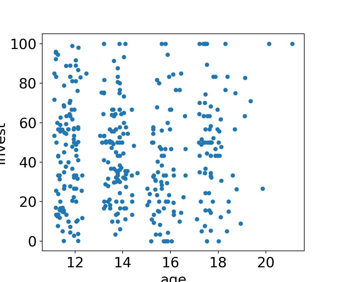
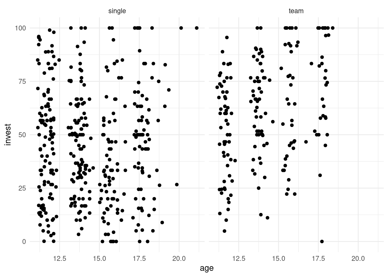
Plot invest ~ age in single and team arrangement:
R
plot(invest ~ age, data = MLA, subset = arrangement == "single", main = "arrangement = single")
plot(invest ~ age, data = MLA, subset = arrangement == "team", main = "arrangement = team")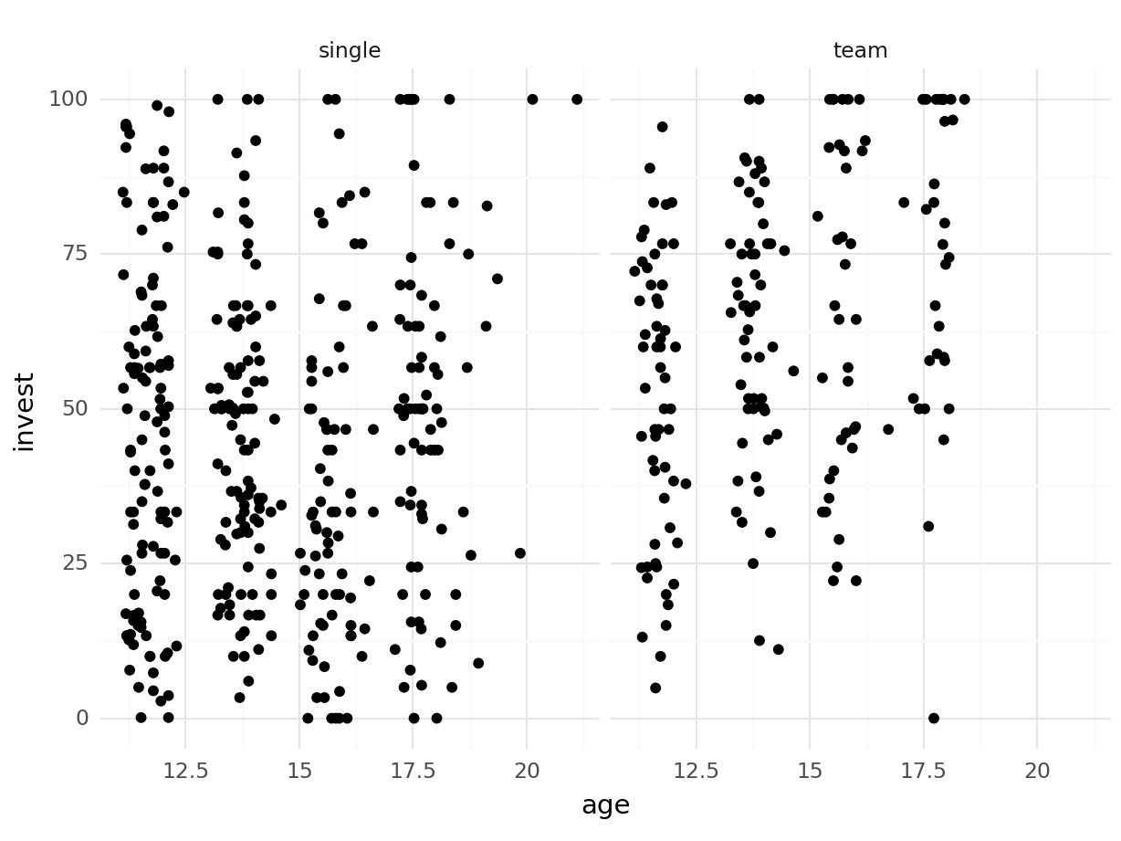

Python
MLA[MLA["arrangement"]=="single"].plot.scatter(x="age", y="invest");
MLA[MLA["arrangement"]=="team"].plot.scatter(x="age", y="invest");
plt.show()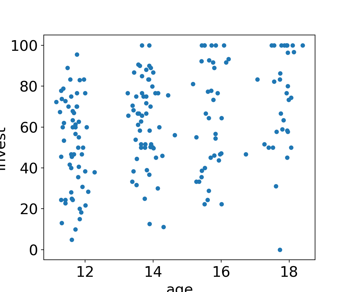
ax = MLA[MLA["arrangement"]=="single"].plot.scatter(x="age", y="invest");
MLA[MLA["arrangement"]=="team"].plot.scatter(x="age", y="invest", ax=ax, c='k');
plt.show()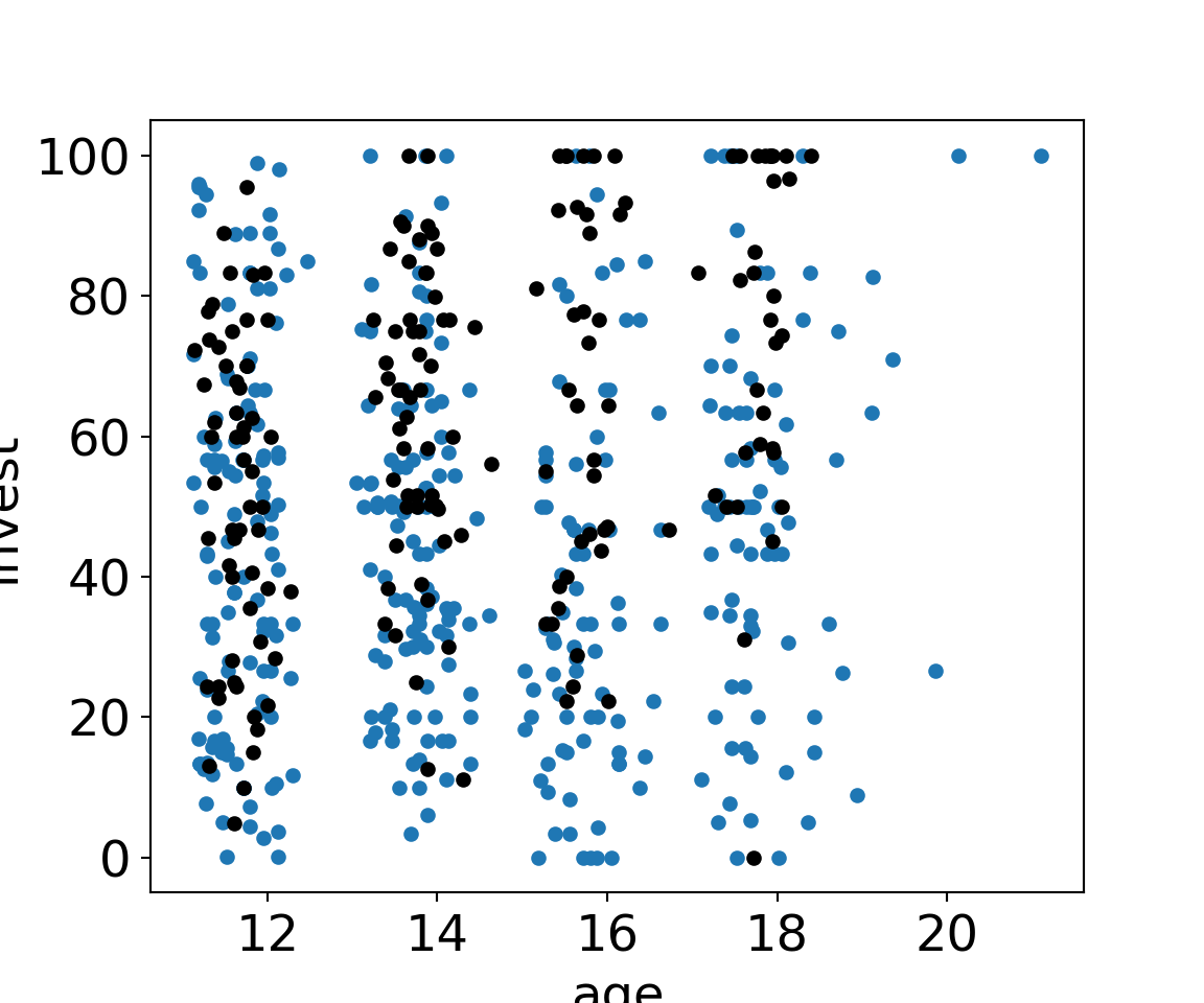
lattice graphics (available in R):
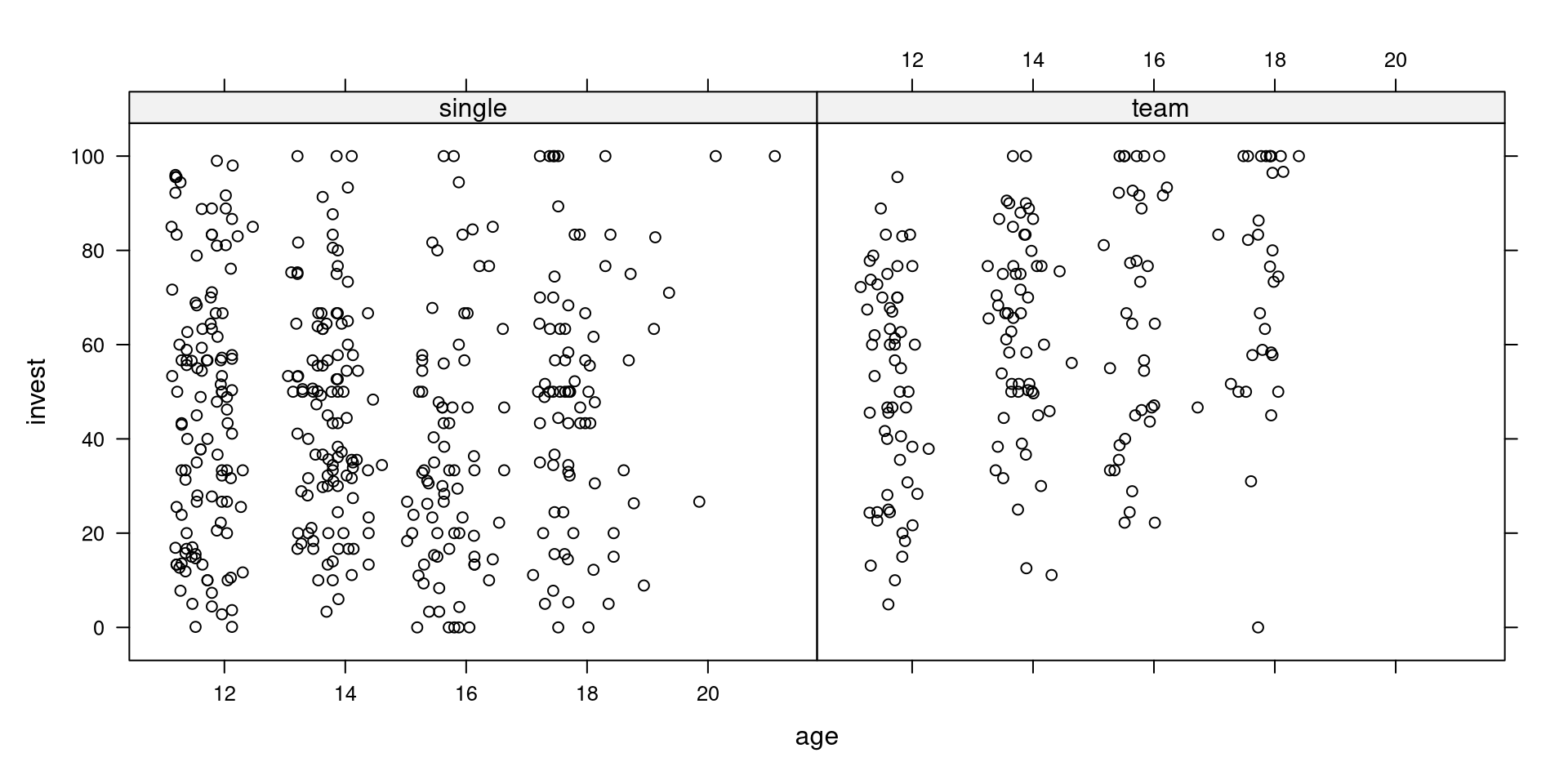
ggplot2 graphics:
Python
ggplot2 graphics (make sure that plotnine is installed):
#from plotnine import ggplot, aes, geom_boxplot, facet_wrap, facet_grid, theme_set, theme_minimal, geom_point, geom_smooth
from plotnine import *

theme_set(theme_minimal());## <string>:1: FutureWarning: Using repr(plot) to draw and show the plot figure is deprecated and will be removed in a future version. Use plot.show().
## <Figure Size: (640 x 480)>
Linear models:
Python
m1 = smf.ols("invest ~ 1", data=MLA).fit()
m_a = smf.ols("invest ~ arrangement", data=MLA).fit()
m_a2 = smf.ols("invest ~ age", data=MLA).fit()
m_aa = smf.ols("invest ~ arrangement + age", data=MLA).fit()
m_aXa = smf.ols("invest ~ arrangement * age", data=MLA).fit()
sm.stats.anova_lm(m1, m_a, m_a2, m_aXa)
## df_resid ssr df_diff ss_diff F Pr(>F)
## 0 569.0 408965.7464 0.0 NaN NaN NaN
## 1 568.0 374810.4899 1.0 34155.2565 53.0760 1.0782e-12
## 2 568.0 405928.1340 -0.0 -31117.6441 inf NaN
## 3 566.0 364230.0586 2.0 41698.0754 32.3986 4.7669e-14Compare models with ANOVA:
R
## Analysis of Variance Table
##
## Model 1: invest ~ 1
## Model 2: invest ~ arrangement
## Model 3: invest ~ arrangement + age
## Model 4: invest ~ arrangement * age
##   Res.Df    RSS Df Sum of Sq     F  Pr(>F)
## 1    569 408966
## 2    568 374810  1     34155 53.08 1.1e-12
## 3    567 370959  1      3851  5.98  0.0147
## 4 566 364230 1 6729 10.46 0.0013## Analysis of Variance Table
##
## Model 1: invest ~ 1
## Model 2: invest ~ age
## Model 3: invest ~ arrangement + age
## Model 4: invest ~ arrangement * age
## Res.Df RSS Df Sum of Sq F Pr(>F)
## 1 569 408966
## 2 568 405928 1 3038 4.72 0.0302
## 3 567 370959 1 34969 54.34 6e-13
## 4 566 364230 1 6729 10.46 0.0013Summary of the model invest ~ arrangement * age
R
##
## Call:
## lm(formula = invest ~ arrangement * age, data = MLA)
##
## Residuals:
##    Min     1Q Median     3Q    Max
## -73.57 -20.81   1.21  18.44  55.17
##
## Coefficients:
##                     Estimate Std. Error t value   Pr(>|t|)
## (Intercept)           42.766      8.045    5.32 0.00000015
## arrangementteam      -29.846     14.584   -2.05     0.0412
## age                    0.156      0.552    0.28     0.7774
## arrangementteam:age    3.266      1.010    3.23     0.0013
##
## Residual standard error: 25.4 on 566 degrees of freedom
## Multiple R-squared:  0.109,  Adjusted R-squared:  0.105
## F-statistic: 23.2 on 3 and 566 DF,  p-value: 3.69e-14
Python
##                             OLS Regression Results
## ==============================================================================
## Dep. Variable:                 invest   R-squared:                       0.109
## Model:                            OLS   Adj. R-squared:                  0.105
## Method:                 Least Squares   F-statistic:                     23.17
## Date:                Wed, 05 Mar 2025   Prob (F-statistic):           3.69e-14
## Time:                        14:23:37   Log-Likelihood:                -2649.9
## No. Observations:                 570   AIC:                             5308.
## Df Residuals:                     566   BIC:                             5325.
## Df Model:                           3
## Covariance Type:            nonrobust
## ===========================================================================================
##                               coef    std err          t      P>|t|      [0.025      0.975]
## -------------------------------------------------------------------------------------------
## Intercept                  42.7662      8.045      5.316      0.000      26.965      58.567
## arrangement[T.team]       -29.8461     14.584     -2.046      0.041     -58.492      -1.200
## age                         0.1561      0.552      0.283      0.777      -0.928       1.240
## arrangement[T.team]:age     3.2661      1.010      3.234      0.001       1.282       5.250
## ==============================================================================
## Omnibus:                       28.763   Durbin-Watson:                   1.562
## Prob(Omnibus):                  0.000   Jarque-Bera (JB):               13.019
## Skew:                           0.129   Prob(JB):                      0.00149
## Kurtosis:                       2.306   Cond. No.                         224.
## ==============================================================================
##
## Notes:
## [1] Standard Errors assume that the covariance matrix of the errors is correctly specified.
Plot invest ~ age in single and team arrangement:
R
plot(invest ~ age, data = MLA, subset = arrangement == "single", main = "arrangement = single")
abline(coef(mAxA)[c(1, 3)], lwd = 2)
plot(invest ~ age, data = MLA, subset = arrangement == "team", main = "arrangement = team")
abline(sum(coef(mAxA)[1:2]), sum(coef(mAxA)[3:4]), lwd = 2)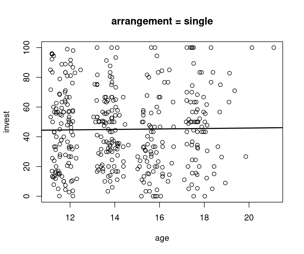
Python
ax = MLA[MLA["arrangement"]=="single"].plot.scatter(x="age", y="invest");
sm.graphics.abline_plot(intercept=m_aXa.params[0], slope=m_aXa.params[2], ax=ax, c="red");
## <string>:1: FutureWarning: Series.__getitem__ treating keys as positions is deprecated. In a future version, integer keys will always be treated as labels (consistent with DataFrame behavior). To access a value by position, use `ser.iloc[pos]`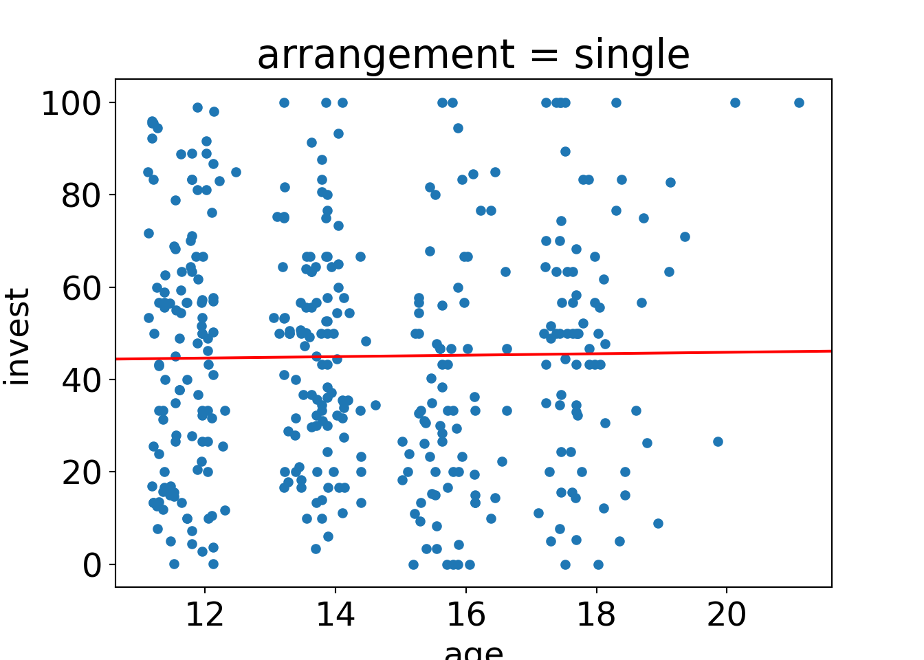
ax = MLA[MLA["arrangement"]=="team"].plot.scatter(x="age", y="invest");
sm.graphics.abline_plot(intercept=np.sum(m_aXa.params[0:2]), slope=np.sum(m_aXa.params[2:4]), ax=ax, c="red");
ax.set_title("arrangement = team")
plt.show()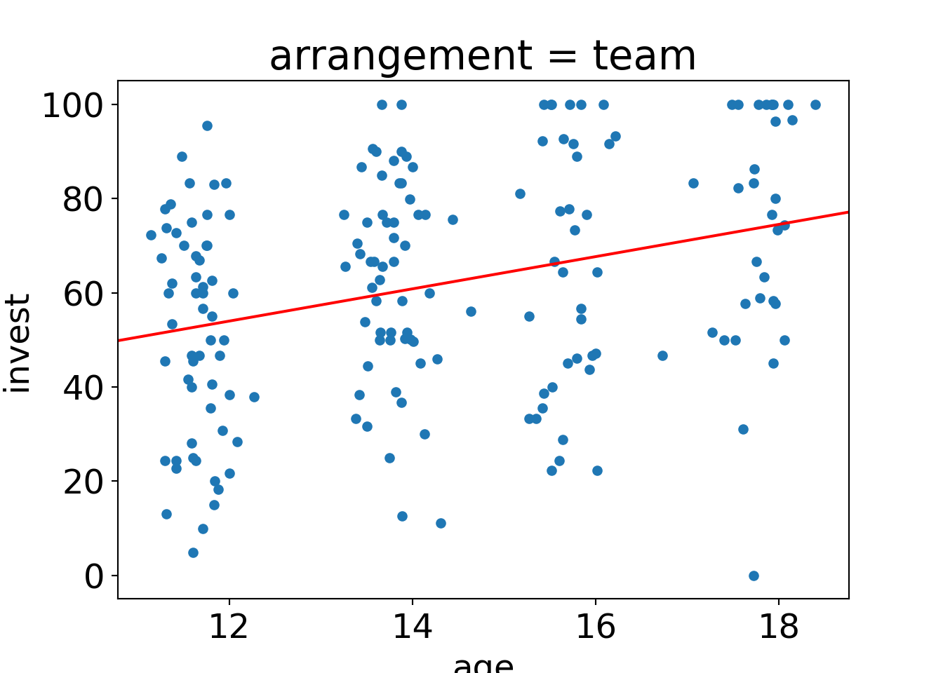
ggplot graphics:
R
ggplot(MLA, aes(x = age, y = invest)) + geom_point() +
  facet_wrap(~ arrangement) + geom_smooth(method = "lm", se = FALSE)
## `geom_smooth()` using formula = 'y ~ x'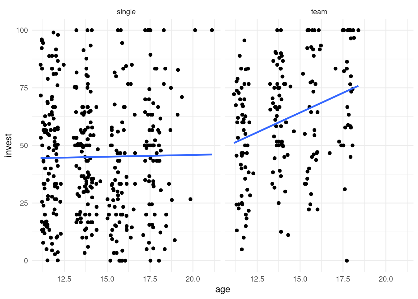
Python
(
    ggplot(MLA, aes(x="age", y="invest")) + geom_point() +
      facet_wrap("~arrangement") + geom_smooth(method="lm", se=False)
)
## <string>:1: FutureWarning: Using repr(plot) to draw and show the plot figure is deprecated and will be removed in a future version. Use plot.show().
## <Figure Size: (640 x 480)>