Chapter 10 Two- and \(k\)-sample analysis of variance
10.1 ANOVA for location differences
Reformulation: The decision between the null hypothesis and alternative hypothesis
\[ \begin{array}{lrcl} H_0: & \mu_A & = & \mu_B \quad (= \mu) \\ H_1: & \mu_A & \neq & \mu_B \end{array} \]
can also be interpreted as a decision between two models (with model error \(\varepsilon\))
\[ \begin{array}{lrcl} M_0: & Y & = & \left. \phantom{\{} \phantom{f} \begin{array}{ll} \mu \phantom{i} + \varepsilon & (\mbox{independent of } X) \end{array} \right. \\ M_1: & Y & = & \left\{ \begin{array}{ll} \mu_A + \varepsilon & \mbox{if } X = A \\ \mu_B + \varepsilon & \mbox{if } X = B \end{array} \right. \end{array} \]
Under \(M_0\): The expectation of \(Y\) is a constant (symbolically: \(Y \sim 1\)). This can be estimated with the empirical mean \(\overline y\). Corresponding residual sum of squares: \[ \mathit{RSS}_0 \quad = \quad \sum_{i = 1}^n (y_i - \overline y)^2 \; = \; (n - 1) \cdot s^2. \]
Under \(M_1\): The expectation of \(Y\) depends on \(X\) (symbolically: \(Y \sim X\)). The group-wise expectations can be estimated with the group-wise empirical means \(\overline y_A\) and \(\overline y_B\), respectively. Corresponding residual sum of squares:
\[\begin{eqnarray*} \mathit{RSS}_1 & = & \sum_{i = 1}^{n_A} (y_{A,i} - \overline y_A)^2 + \sum_{i = 1}^{n_B} (y_{B,i} - \overline y_B)^2 \\ & = & (n_A - 1) \cdot s_A^2 + (n_B - 1) \cdot s_B^2. \end{eqnarray*}\]
Note: The simpler model \(M_0\) is a special case of the more complex model \(M_1\), namely for the case where \(\mu_A = \mu_B\) (under \(H_0\)).
Because \(M_0\) is a special case of \(M_1\) (also: is nested in \(M_1\)), the residual sum of squares (RSS) of \(M_1\) can only be smaller, i.e., \(\mathit{RSS}_1 \le \mathit{RSS}_0\).
Question: Is \(\mathit{RSS}_1\) clearly smaller than \(\mathit{RSS}_0\) or just “a little”?
Idea: Consider the difference \(\mathit{RSS}_0 - \mathit{RSS}_1\).
- \(H_0\) is correct: Both models fit similarly well and the RSS difference is small, i.e., close to 0.
- \(H_1\) is correct: Model \(M_1\) fits substantially better and the RSS difference is large.
10.2 \(F\)-test
Question: When is the difference \(\mathit{RSS}_0 - \mathit{RSS}_1\) “large”?
Answer: Standardize the difference with a dispersion measure, i.e., here the variance \(\hat \sigma^2 = \mathit{RSS}_1 / (n - 2)\) under the alternative \(H_1\).
\[\begin{equation*} F ~=~ \frac{\mathit{RSS}_0 - \mathit{RSS}_1}{\mathit{RSS}_1 / (n - 2)}. \end{equation*}\]
Reject \(H_0\) if \(F\) becomes greater than the corresponding critical value at significance level \(\alpha\).
Null distribution: Under \(H_0\) (and assuming normally distributed errors \(\varepsilon\)) the \(F\)-statistic is \(F\)-distributed with 1 and \(n - 2\) degrees of freedom. For increasing \(n\) the \(F_{1, n-2}\)-distribution converges to a \(\chi^2_1\)-distribution with 1 degree of freedom.
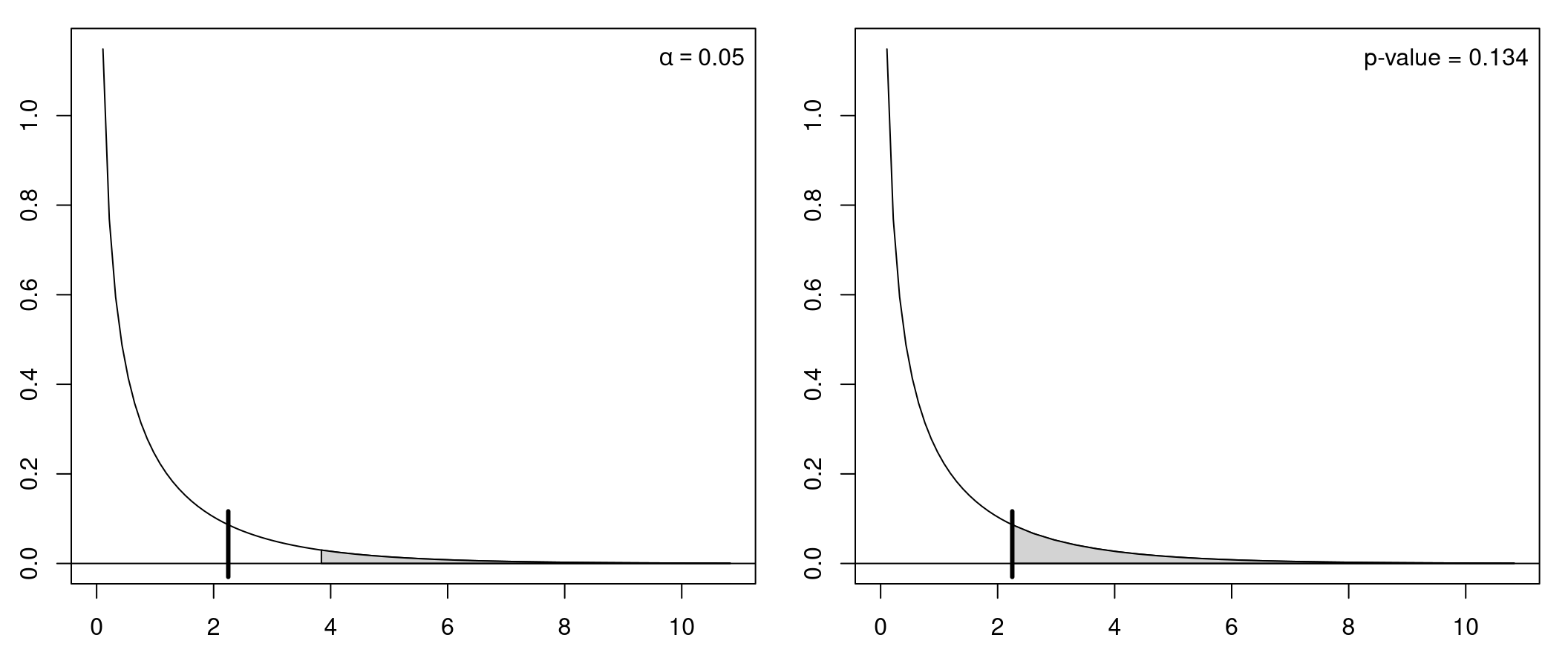
Figure 10.1: F-test: Based on critical value (left) or p-value (right)
Illustration: Artificial 2-sample data without location difference (dat_noshift) and with location difference (dat_shift), respectively.
Idea: Under the null hypothesis (\(Y \sim~ 1\)), the location of the two samples does not differ. Thus, it makes no (or not much) difference whether the location and dispersion is estimated only once in the overall sample or separately for the two samples. However, under the alternative (\(Y \sim~ X\)) the dispersion around separate locations in the two samples will be much smaller.
Visualization: Parallel boxplots as in plot(y ~ x, data = dat_noshift).
10.3 ANOVA table
Res. Df. |
RSS |
Df. |
Sum of Sq. |
F |
Pr(>F) |
|
|---|---|---|---|---|---|---|
1 |
\(n - 1\) | \(\mathit{RSS}_0\) | ||||
2 |
\(n - 2\) | \(\mathit{RSS}_1\) | 1 | \(\mathit{RSS}_0-\mathit{RSS}_1\) | \(F\) | \(p\)-value |
Analysis of variance: \(F\)-tests are often conducted schematically in an analysis of variance (ANOVA).
ANOVA table: Summary of the most important information from both models along with their differences.
Res. Df. |
RSS |
Df. |
Sum of Sq. |
F |
Pr(>F) |
|
|---|---|---|---|---|---|---|
1 |
\(79\) | \(67.41\) | ||||
2 |
\(78\) | \(67.35\) | \(1\) | \(0.1\) | \(0.1\) | \(0.8034\) |
Coefficient of determination: Here, the proportion of variance explained in addition by the variable \(X\) is
\[\begin{eqnarray*} \frac{\mathit{RSS}_0 - \mathit{RSS}_1}{\mathit{RSS}_0} ~=~ \frac{67.41 - 67.35}{67.41} ~=~ \frac{0.1}{67.41} ~=~ 0.001. \end{eqnarray*}\]
ANOVA table:
Res. Df. |
RSS |
Df. |
Sum of Sq. |
F |
Pr(>F) |
|
|---|---|---|---|---|---|---|
1 |
\(79\) | \(774.95\) | ||||
2 |
\(78\) | 67.35 | \(1\) | \(707.6\) | \(819.5\) | 0 |
Coefficient of determination: Here, the proportion of variance explained in addition by the variable \(X\) is
\[\begin{eqnarray*} \frac{\mathit{RSS}_0 - \mathit{RSS}_1}{\mathit{RSS}_0} ~=~ \frac{774.95 - 67.35}{774.95} ~=~ \frac{707.6}{774.95} ~=~ 0.913. \end{eqnarray*}\]
10.4 Example
Example: Dependence of invest on arrangement in MLA data.
## Analysis of Variance Table
##
## Model 1: invest ~ 1
## Model 2: invest ~ arrangement
##   Res.Df    RSS Df Sum of Sq     F   Pr(>F)
## 1    569 408966
## 2    568 374810  1     34155 51.76 1.99e-12
Building blocks: Computation based on groupwise statistics.
\[\begin{eqnarray*} \mathit{RSS}_0 & = & \sum_{i = 1}^n (y_i - \overline y)^2 \\ & = & (n - 1) \cdot s^2 \\ & = & (570 - 1) \cdot 26.8^2 \\ & = & 408965.7 \\ \mathit{RSS}_1 & = & \sum_{i = 1}^{n_\mathsf{Single}} (y_{\mathsf{Single},i} - \overline y_\mathsf{Single})^2 ~+~ \sum_{i = 1}^{n_\mathsf{Team}} (y_{\mathsf{Team},i} - \overline y_\mathsf{Team})^2 \\ & = & (n_\mathsf{Single} - 1) \cdot s_\mathsf{Single}^2 ~+~ (n_\mathsf{Team} - 1) \cdot s_\mathsf{Team}^2 \\ & = & (385 - 1) \cdot 26.2^2 ~+~ (185 - 1) \cdot 24.5^2 \\ & = & 374810.5 \end{eqnarray*}\]
Subsequently: Compute \(F\)-statistics and coefficient of determination.
\[\begin{eqnarray*} F & = & \frac{(\mathit{RSS}_0 - \mathit{RSS}_1)/(k - 1)}{\mathit{RSS}_1/(n-2)} \\ & = & \frac{(408965.7 - 374810.5)/1}{374810.5/(570 - 2)} \\ & = & 51.8 \\ R^2 & = & 1 - \frac{\mathit{RSS}_1}{\mathit{RSS}_0} \\ & = & 1 - \frac{374810.5}{408965.7} \\ & = & 0.084. \end{eqnarray*}\]
In R:
##
##  One-way analysis of means
##
## data:  invest and arrangement
## F = 51.76, num df = 1, denom df = 568, p-value = 1.99e-12##
## One-way analysis of means
##
## data: invest and treatment
## F = 1.61, num df = 1, denom df = 568, p-value = 0.205Remark: Analogously to the \(t\)-test there is a version of the \(F\)-test that is computed without the assumption of equal variances.
10.5 \(F\)-test vs. \(t\)-test
Surprise: The \(F\)-test yields exactly the same \(p\)-value as the two-sided \(t\)-test. Also the test statistics are closely related: \(F = 1.61 = (-1.269)^2 = t^2\).
Generally: In the 2-sample case the \(F\)-test and (two-sided) \(t\)-test are equivalent with \(F = t^2\).
Question: Why the hassle? The \(t\)-test is intuitive and easy to interpret. Why go through the trouble of constructing a second test that ends up being equivalent?
Answer: The \(F\)-test is more versatile. While the \(t\)-test only works for the comparison of means from two samples, the ANOVA can be applied to the comparison of \(k\) samples in exactly the same way as before.
10.6 ANOVA for \(k\)-sample differences
Hypotheses:
\[ \begin{array}{ll} H_0: & \mbox{Expectations in all subsamples are equal} \\ & \mu_A = \mu_B = \mu_C = \dots \\ H_1: & \mbox{Expectation in at least one subsample differs.} \end{array} \]
ANOVA: Compare the null model with one overall mean (as before) with the alternative model with \(k\) means for the \(k\) subsamples.
Res. Df. |
RSS |
Df. |
Sum of Sq. |
F |
Pr(>F) |
|
|---|---|---|---|---|---|---|
1 |
\(n - 1\) | \(\mathit{RSS}_0\) | ||||
2 |
\(n - k\) | \(\mathit{RSS}_1\) | \(k-1\) | \(\mathit{RSS}_0-\mathit{RSS}_1\) | \(F\) | \(p\)-value |
\(F\)-test: Under \(H_0\) the corresponding \(F\)-statistic is \(F\)-distributed with \(k - 1\) and \(n - k\) degrees of freedom (under normality), or \((k - 1) \cdot F\) is asymptotically \(\chi^2_{k - 1}\)-distributed.
\[\begin{equation*} F ~=~ \frac{(\mathit{RSS}_0 - \mathit{RSS}_1)/(k - 1)}{\mathit{RSS}_1 / (n - k)}. \end{equation*}\]
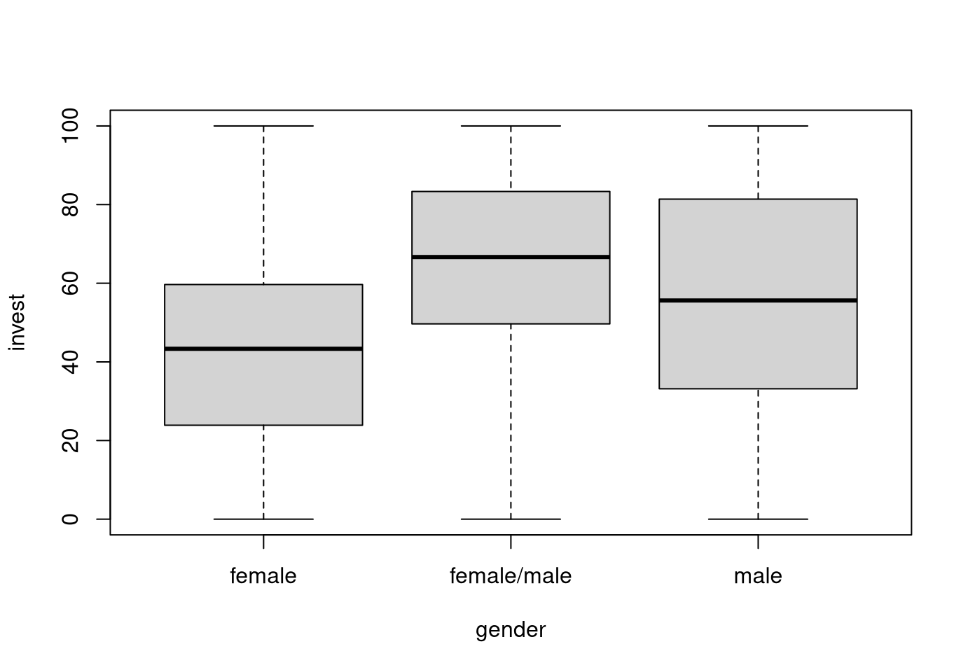
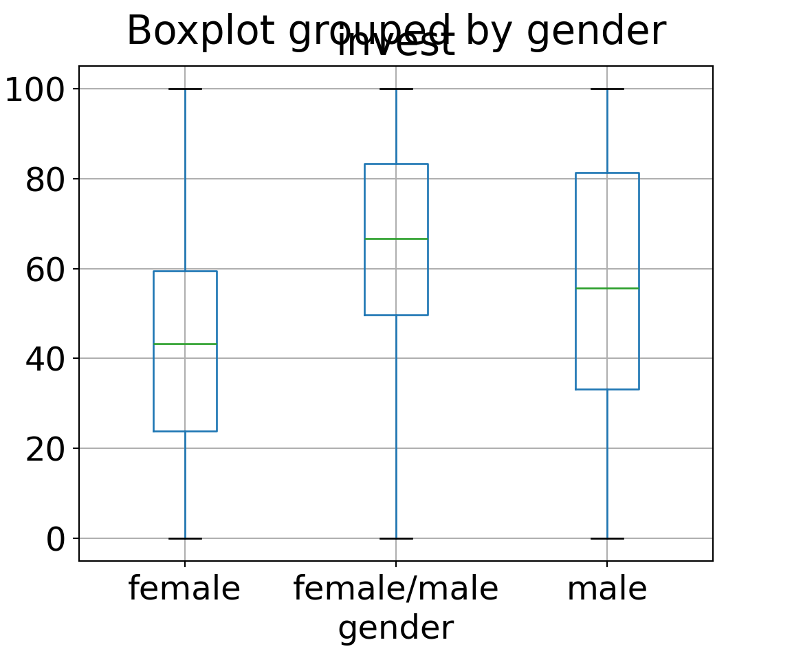
Example: Dependence of invest on gender in MLA data.
Groupwise statistics:
| Female | Female/male | Male | Overall | |
|---|---|---|---|---|
| \(n\) | 320 | 86 | 164 | 570 |
| \(\overline y\) | 43.6 | 65.4 | 55.8 | 50.4 |
| \(s\) | 24.2 | 23.5 | 28.9 | 26.8 |
ANOVA:
## Analysis of Variance Table
##
## Model 1: invest ~ 1
## Model 2: invest ~ gender
##   Res.Df    RSS Df Sum of Sq    F   Pr(>F)
## 1    569 408966
## 2    567 369947  2     39018 29.9 4.51e-13
10.7 Tutorial
10.7.1 Setup
Load the MLA data set. (The data set can be downloaded as MLA.csv or MLA.rda.)
R
##    invest      gender male     age treatment grade arrangement
## 1 70.0000 female/male  yes 11.7533      long   6-8        team
## 2 28.3333 female/male  yes 12.0866      long   6-8        team
## 3 50.0000 female/male  yes 11.7950      long   6-8        team
Python
# Make sure that the required libraries are installed.
# Import the necessary libraries and classes:
import pandas as pd
import numpy as np
from matplotlib import pyplot as plt
import seaborn as sns

pd.set_option("display.precision", 4) # Set display precision to 4 digits in pandas and numpy.
# Load dataset
MLA = pd.read_csv("MLA.csv", index_col=False, header=0)
# Preview the first 5 lines of the loaded data
MLA.head()## invest gender male age treatment grade arrangement
## 0 70.0000 female/male yes 11.7533 long 6-8 team
## 1 28.3333 female/male yes 12.0866 long 6-8 team
## 2 50.0000 female/male yes 11.7950 long 6-8 team
## 3 50.0000 male yes 13.7566 long 6-8 team
## 4 24.3333 female/male yes 11.2950 long 6-8 team10.7.2 2-sample ANOVA
Using the \(F\)-test from an analysis of variance (ANOVA) for the 2-sample test yields the same \(p\)-value as in the 2-sided \(t\)-test. The test statistic is simply \(F = t^2\).
Compared to the 2-sample \(t\)-test the \(F\)-test from the ANOVA has the advantage that it naturally extends to \(k\) samples as well. The disadvantage is that only two-sided alternatives can be assessed. As for the \(t\)-test there is a version that assumes equal variances and a version that does not.
R
In R one option to conduct this \(F\)-test is the function oneway.test():
##
##  One-way analysis of means
##
## data:  invest and arrangement
## F = 51.76, num df = 1, denom df = 568, p-value = 1.99e-12##
## One-way analysis of means
##
## data: invest and treatment
## F = 1.61, num df = 1, denom df = 568, p-value = 0.205Python
Using the function anova_oneway() from statsmodels.
Note that the function returns the \(F\)-score named statistic.
from statsmodels.stats.oneway import anova_oneway

res = anova_oneway(data=MLA["invest"], groups=MLA["arrangement"], use_var='equal', welch_correction=False)
print(res)
## statistic = 51.7599859849463
## pvalue = 1.991313440338478e-12
## df = (1.0, np.float64(568.0))
## df_num = 1.0
## df_denom = 568.0
## nobs_t = 570.0
## n_groups = 2
## means = [45.01240952 61.54534514]
## nobs = [385. 185.]
## vars_ = [688.60938672 599.91568145]
## use_var = equal
## welch_correction = False
## tuple = (np.float64(51.7599859849463), np.float64(1.991313440338478e-12))res = anova_oneway(data=MLA["invest"], groups=MLA["treatment"], use_var='equal', welch_correction=False)
print(res)## statistic = 1.609797543284716
## pvalue = 0.20503996927043125
## df = (1.0, np.float64(568.0))
## df_num = 1.0
## df_denom = 568.0
## nobs_t = 570.0
## n_groups = 2
## means = [48.95438541 51.80233921]
## nobs = [285. 285.]
## vars_ = [710.24556376 725.70497001]
## use_var = equal
## welch_correction = False
## tuple = (np.float64(1.609797543284716), np.float64(0.20503996927043125))10.7.3 \(k\) samples
To show that the \(F\)-test from an ANOVA can also be applied easily to a
\(k\)-sample problem, we consider testing for gender differences in invest
levels in the MLA data. The exploratory display using parallel boxplots
shows that female players (both single or teams) have somewhat lower investments
than male players (both single or teams) and mixed female/male teams.

Note that these gender labels are intertwined with the arrangement
because gender = "female/male" implies arrangement = "team". Therefore,
the following tests of gender effects are always confounded with the significant
arrangement effects found above. To disentangle the effects an analysis with
linear models will be considered in the next chapter.
In any case, putting these considerations aside for a moment, we can employ the following \(F\)-tests as an illustration for location differences in \(k\) samples (here with \(k = 3\)):
R
##
##  One-way analysis of means
##
## data:  invest and gender
## F = 29.9, num df = 2, denom df = 567, p-value = 4.51e-13##
## One-way analysis of means (not assuming equal variances)
##
## data: invest and gender
## F = 32.88, num df = 2.0, denom df = 217.1, p-value = 3.37e-13Python
res = anova_oneway(data=MLA["invest"], groups=MLA["gender"], use_var='equal', welch_correction=False)
print(res)
## statistic = 29.900805622211355
## pvalue = 4.512452663095832e-13
## df = (2.0, np.float64(567.0))
## df_num = 2.0
## df_denom = 567.0
## nobs_t = 570.0
## n_groups = 3
## means = [43.56562458 65.36950884 55.81029812]
## nobs = [320. 86. 164.]
## vars_ = [584.05256376 554.09394077 837.64767073]
## use_var = equal
## welch_correction = False
## tuple = (np.float64(29.900805622211355), np.float64(4.512452663095832e-13))res = anova_oneway(data=MLA["invest"], groups=MLA["gender"], use_var='unequal', welch_correction=False)
print(res)## statistic = 32.9783952108139
## pvalue = 3.1165868362301765e-13
## df = (2.0, np.float64(217.08112642531304))
## df_num = 2.0
## df_denom = 217.08112642531304
## nobs_t = 570.0
## n_groups = 3
## means = [43.56562458 65.36950884 55.81029812]
## nobs = [320. 86. 164.]
## vars_ = [584.05256376 554.09394077 837.64767073]
## use_var = unequal
## welch_correction = False
## tuple = (np.float64(32.9783952108139), np.float64(3.1165868362301765e-13))This shows that mean investments vary significantly across the gender samples.