Chapter 14 Analysis of variance
14.1 1-way analysis of variance
So far: Quantitative variables \(x_{ij}\) as regressors.
\[\begin{eqnarray*} y_i & = & \beta_1 ~+~ \beta_2 \cdot x_{i2} ~+~ \dots ~+~ \beta_k \cdot x_{ik} ~+~ \varepsilon_i \\ y_i & = & x_i^\top \beta ~+~ \varepsilon_i \\ \text{E}(y_i) ~=~ \mu_i & = & x_i^\top \beta \end{eqnarray*}\]
Question: How to include qualitative variables that affect \(y_i\)?
Known: The influence of a qualitative explanatory variable only can be assessed with the 2-sample \(t\)-test or \(k\)-sample \(F\)-test.
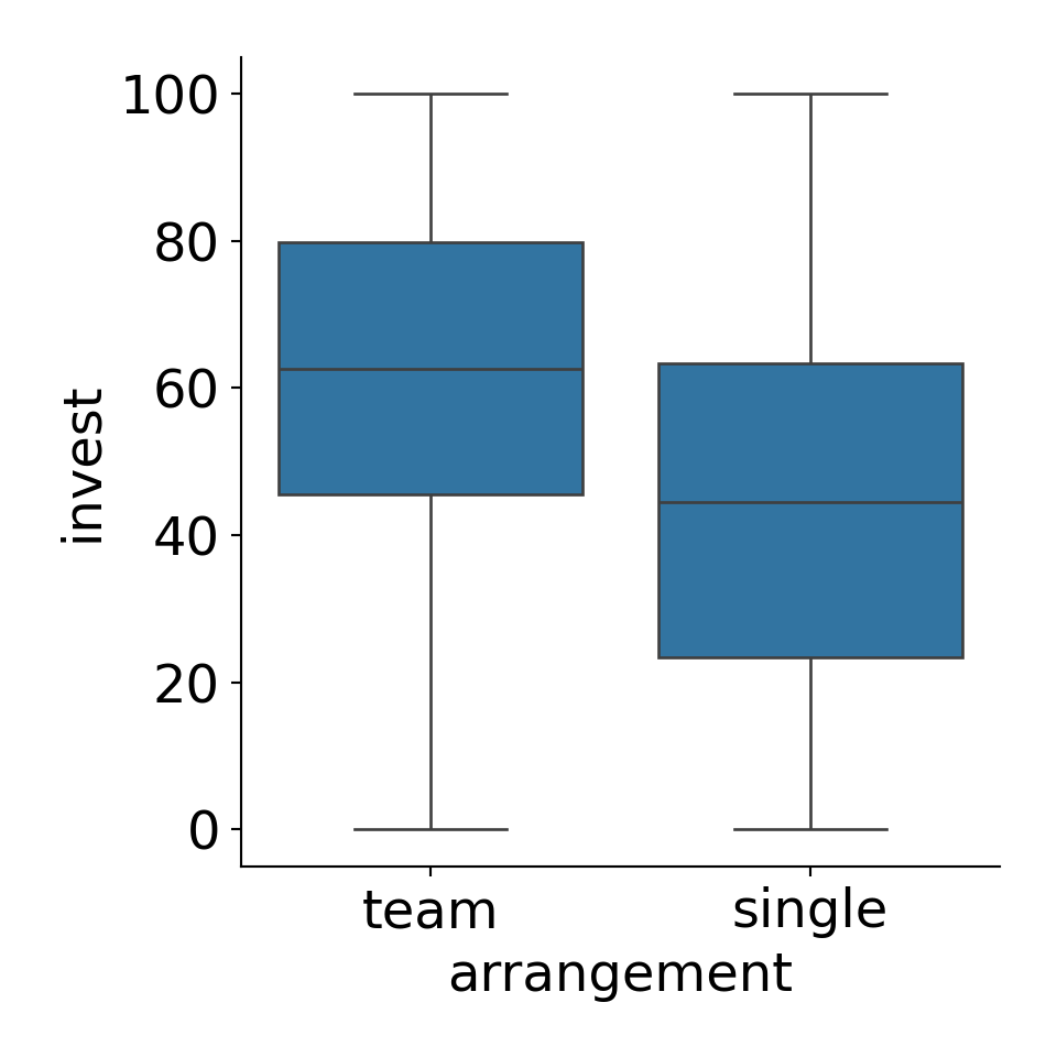
Example: Dependence of investments on arrangement in MLA experiment. The empirical means are \(45.012\) (single) and \(61.545\) (team).
Visualization:
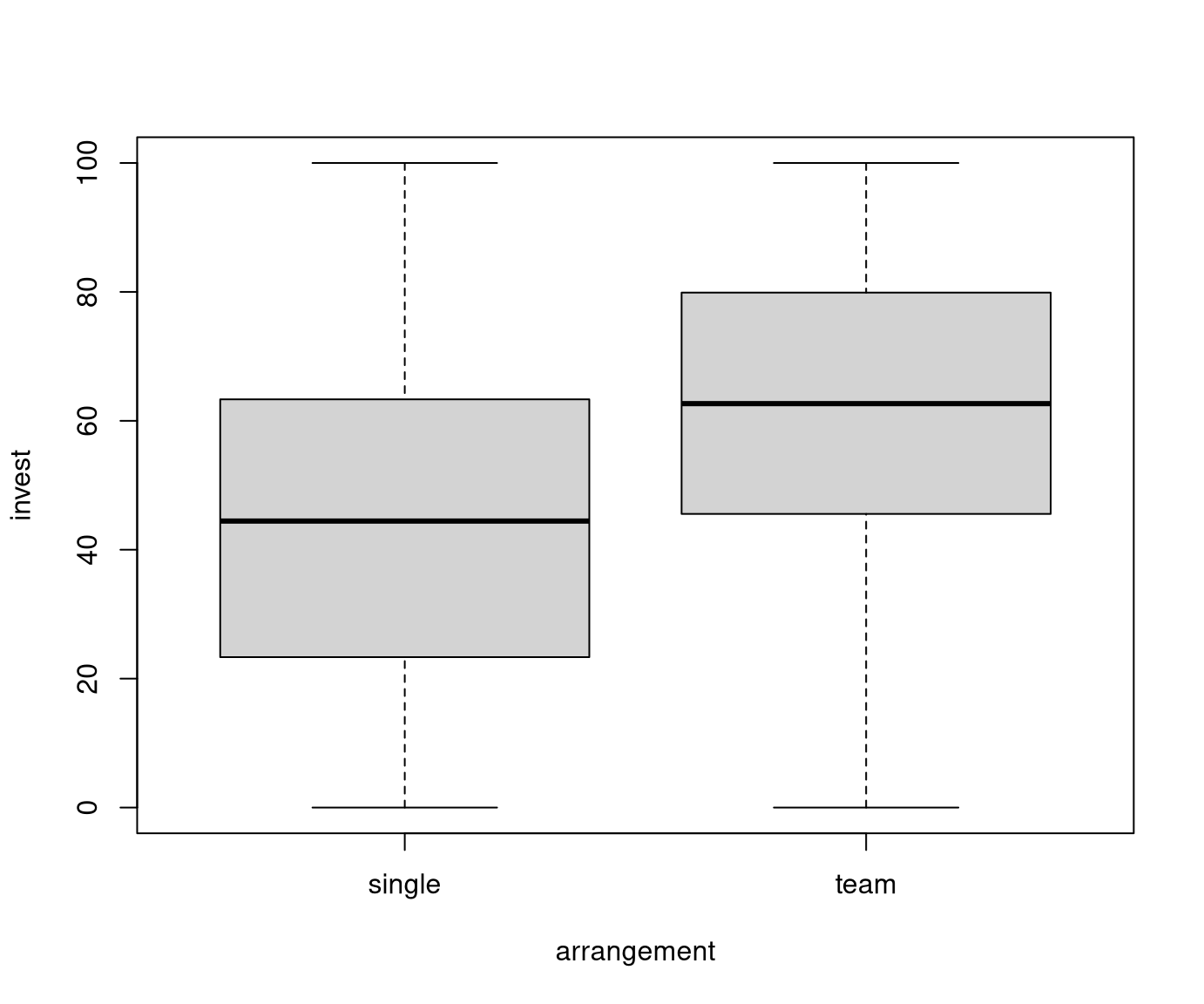
Wanted: Linear regression model for which the corresponding \(t\)-test and \(F\)-test coincide with the known tests.
Problem: To include arrangement in the linear regression model, the categorical observations (single, single, team, single, team, \(\dots)^\top\) need to be turned into some numerical regressor(s) \(x_{ij}\).
Idea: Generate two so-called indicator variables (or dummy variables) which indicate whether a particular observations falls into the single category \(x_{i2} = (1, 1, 0, 1, 0, \dots)^\top\) or team category \(x_{i3} = (0, 0, 1, 0, 1, \dots)^\top\). The regression equation is then
\[ y_i \quad = \quad \beta_1 ~+~ \beta_2 \cdot x_{i2} ~+~ \beta_3 \cdot x_{i3} ~+~ \varepsilon_i. \]
Matrix notation:
\[\begin{equation*} \left( \begin{array}{c} y_1 \\ y_2 \\ y_3 \\ y_4 \\ y_5 \\ \vdots \\ \end{array} \right) \quad = \quad \left(\begin{array}{ccc} 1 & 1 & 0 \\ 1 & 1 & 0 \\ 1 & 0 & 1 \\ 1 & 1 & 0 \\ 1 & 0 & 1 \\ & \vdots & \end{array} \right) ~ \left( \begin{array}{c} \beta_1 \\ \beta_2 \\ \beta_3 \\ \end{array} \right) ~+~ \left( \begin{array}{c} \varepsilon_1 \\ \varepsilon_2 \\ \varepsilon_3 \\ \varepsilon_4 \\ \varepsilon_5 \\ \vdots \\ \end{array} \right) \end{equation*}\]
Problem: This regressor matrix \(X\) violates a basic assumption.
- A5: No linear dependencies: \(\mathsf{rank}(X) = k\).
Here: \(\mathsf{rank}(X) = 3\) would be needed. However, there is a rather obvious linear dependency. The first column (intercept) is the sum of the two columns (indicator variables).
Hence: \(\mathsf{rank}(X) = 2\). And thus only two (rather than three) parameters can be estimated for determining the mean of \(y\).
Note: This corresponds to our first intuition to estimate two means for the two subsamples.
14.1.1 Contrasts: 1-way Analysis of Variance
Solution: Make the model identifiable by introducing a linear restriction for the original parameters
- \(\beta_1 =\) intercept,
- \(\beta_2 =\) single effect,
- \(\beta_3 =\) team effect.
Options: Among others,
- \(\beta_1 = 0\),
- \(\beta_2 = 0\),
- \(\beta_2 + \beta_3 = 0\).
Jargon: Restrictions that pertain only to the coefficients of the qualitative variable (here: \(\beta_2\), \(\beta_3\)) are also known as contrasts.
First: The restriction \(\beta_1 = 0\) omits the intercept. Then the remaining estimators are simply the group means. \[ \hat \beta_2 = 45.012, \quad \hat \beta_3 = 61.545. \]
However: The group means themselves are not the main focus but rather their difference (and whether this is significant).
Hence: The contrast \(\beta_2 = 0\) is more commonly used, leading to \[ \hat \beta_1 = 45.012, \quad \hat \beta_3 = 16.533. \]
Interpretation: The intercept \(\hat \beta_1\) yields the mean in the single arrangement (reference category). The team arrangement effect \(\hat \beta_3\) is the difference between the two arrangements.
Moreover: The regression model also provides the standard errors for all coefficients. \(\widehat{\mathit{SD}(\hat \beta_3)} = 2.298\) corresponds to the pooled estimate.
Thus: The marginal \(t\)-test assessing the significance of \(\hat \beta_3\) (i.e., \(\beta_3 = 0\) vs. \(\beta_3 \neq 0\)) is the standard 2-sample \(t\)-test that assesses whether invest depends on arrangement.
Jargon: These contrasts are known as treatment contrasts, where the effect in the reference category is restricted to 0.
##
## Call:
## lm(formula = invest ~ arrangement, data = MLA)
##
## Residuals:
##    Min     1Q Median     3Q    Max
## -61.55 -19.77  -0.01  18.32  54.99
##
## Coefficients:
##                 Estimate Std. Error t value Pr(>|t|)
## (Intercept)        45.01       1.31   34.38   <2e-16
## arrangementteam    16.53       2.30    7.19    2e-12
##
## Residual standard error: 25.7 on 568 degrees of freedom
## Multiple R-squared:  0.0835, Adjusted R-squared:  0.0819
## F-statistic: 51.8 on 1 and 568 DF,  p-value: 1.99e-12
Remark: The fitted/predicted values from the model do not depend on the contrasts applied. They are always given by the group means.
\(F\)-test: The \(F\)-test that assesses whether invest depends on arrangement is also known as 1-way analysis of variance.
## Analysis of Variance Table
##
## Model 1: invest ~ 1
## Model 2: invest ~ arrangement
##   Res.Df    RSS Df Sum of Sq    F Pr(>F)
## 1    569 408966
## 2    568 374810  1     34155 51.8  2e-12
Extension: For more than 2 samples (i.e., a qualitative explanatory variable with more than 2 categories) the same ideas can be applied.
However: \(t\)-tests and \(F\)-test then do not test the same null hypothesis.
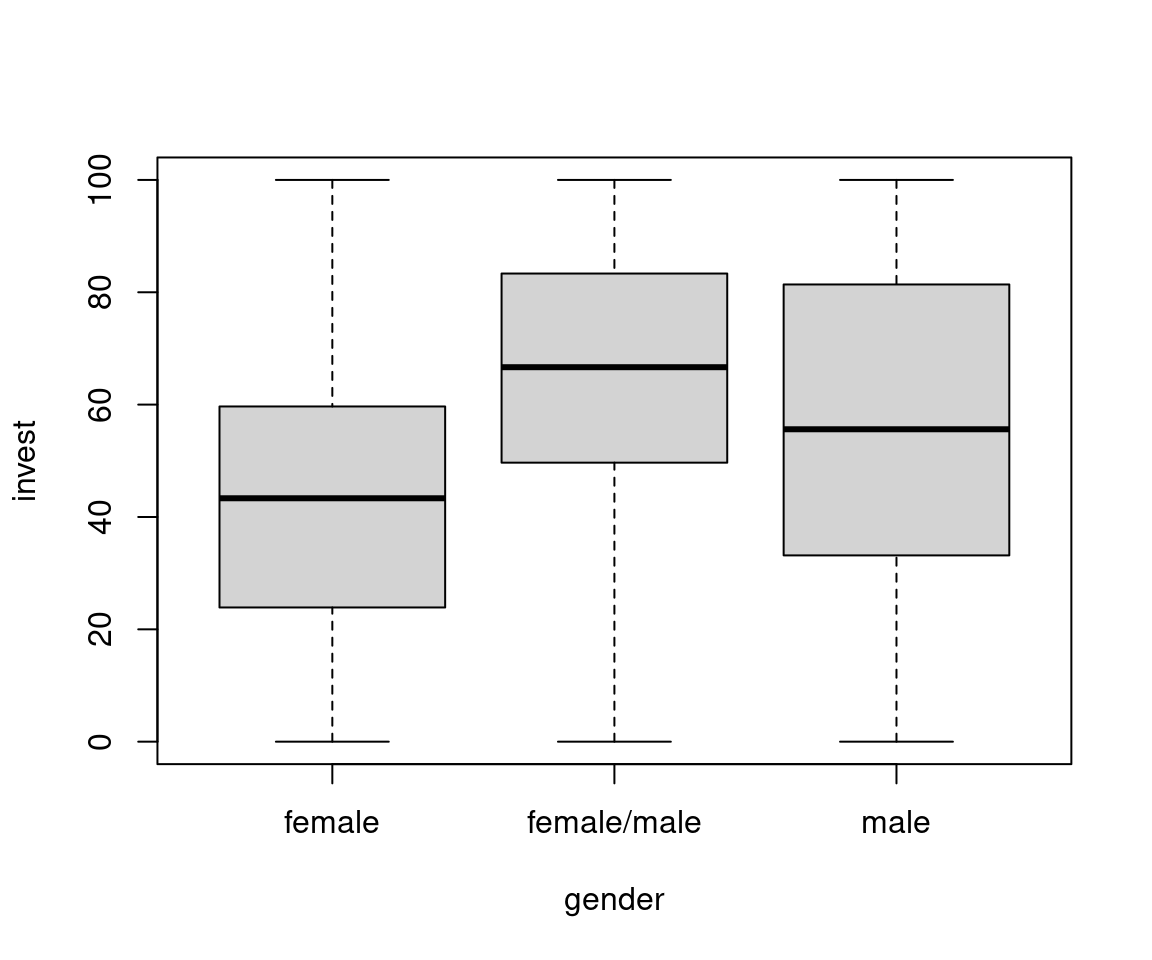
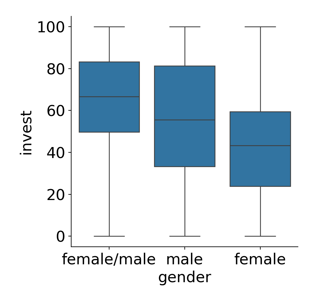
Example: Dependence of invest on gender.
Groupwise statistics:
| Female | Female/Male | Male | Overall | |
|---|---|---|---|---|
| \(n\) | 320 | 86 | 164 | 570 |
| \(\overline y\) | 43.57 | 65.37 | 55.81 | 50.38 |
| \(s\) | 24.17 | 23.54 | 28.94 | 26.81 |
ANOVA:
## Analysis of Variance Table
##
## Model 1: invest ~ 1
## Model 2: invest ~ gender
##   Res.Df    RSS Df Sum of Sq    F  Pr(>F)
## 1    569 408966
## 2    567 369947  2     39018 29.9 4.5e-13
Remarks:
- Fitted/predicted values are not affected by contrasts.
- Hence, residual sums of squares are not affected and consequently ANOVA and \(F\)-test remain the same.
- Only the coding of the coefficients \(\beta\) changes and consequently the corresponding \(t\)-tests.
In R: Treatment contrasts are employed for factor variables by default, using the first category as reference category if not specified otherwise (here: male).
Consequently:
- \(\beta_1\) provides the expectation in the reference category.
- The other coefficients \(\beta_j\) (\(j \ge 2\)) correspond to expected differences of category \(j\) and the reference category, respectively.
##
## Call:
## lm(formula = invest ~ gender, data = MLA)
##
## Residuals:
##    Min     1Q Median     3Q    Max
## -65.37 -20.34   0.08  19.77  56.43
##
## Coefficients:
##                   Estimate Std. Error t value Pr(>|t|)
## (Intercept)          43.57       1.43   30.51   <2e-16
## genderfemale/male    21.80       3.10    7.03    6e-12
## gendermale           12.24       2.45    4.99    8e-07
##
## Residual standard error: 25.5 on 567 degrees of freedom
## Multiple R-squared:  0.0954, Adjusted R-squared:  0.0922
## F-statistic: 29.9 on 2 and 567 DF,  p-value: 4.51e-13
Interpretation:
- Overall, investment depends significantly on gender (\(F = 29.9\), \(p < 0.001\)).
- Expected investment for female players (single or team):
\[\begin{eqnarray*} \hat y_\mathsf{Female} & = & \hat \beta_1 \cdot 1 + \hat \beta_2 \cdot 0 + \hat \beta_3 \cdot 0 \\ & = & \hat \beta_1 \\ & = & 43.57. \end{eqnarray*}\]
- Expected investment for male players (single or team):
\[\begin{eqnarray*} \hat y_\mathsf{Male} & = & \hat \beta_1 \cdot 1 + \hat \beta_2 \cdot 0 + \hat \beta_3 \cdot 1 \\ & = & \hat \beta_1 ~+~ \hat \beta_3 \\ & = & 55.81. \end{eqnarray*}\]
- The difference in investments is thus:
\[\begin{eqnarray*} 55.81 - 43.57 & = & (\hat \beta_1 + \hat \beta_3) - \hat \beta_1 \\ & = & \hat \beta_3 \\ & = & 12.24. \end{eqnarray*}\]
Thus, the expected investments for male players are 12.24 percentage points higher than for female players.
- The difference in expected investments between male and female players is significant as \(\hat \beta_3\) differs significantly from 0 (\(t = 4.99\), \(p < 0.001\)).
Moreover: Analogous interpretation for \(\beta_2\) that estimates the expected difference between mixed teams of female/male players and female players only.
Remark: The effect of the gender variable is a bit tricky to interpret because it combines the gender information with the arrangement (single vs. team). Subsequently, the effect of a male indicator along with the arrangement variable will be considered.
14.2 2-way analysis of variance
Previously: Ideas in the 1-way analysis of variance.
- One explanatory qualitative variable with \(k\) categories.
- Dependent variable can be split into \(k\) samples with corresponding means.
- Contrasts can be applied to suitably code effects for parameters of interest.
Question: What to do with two qualitative explanatory variables with \(k\) and \(\ell\) categories, respectively?
Answer: The dependent variable can be split into up to \(k \cdot \ell\) subsamples, formed by the combination of both explanatory variables.
Consequently: Up to \(k \cdot \ell\) parameters can be estimated.
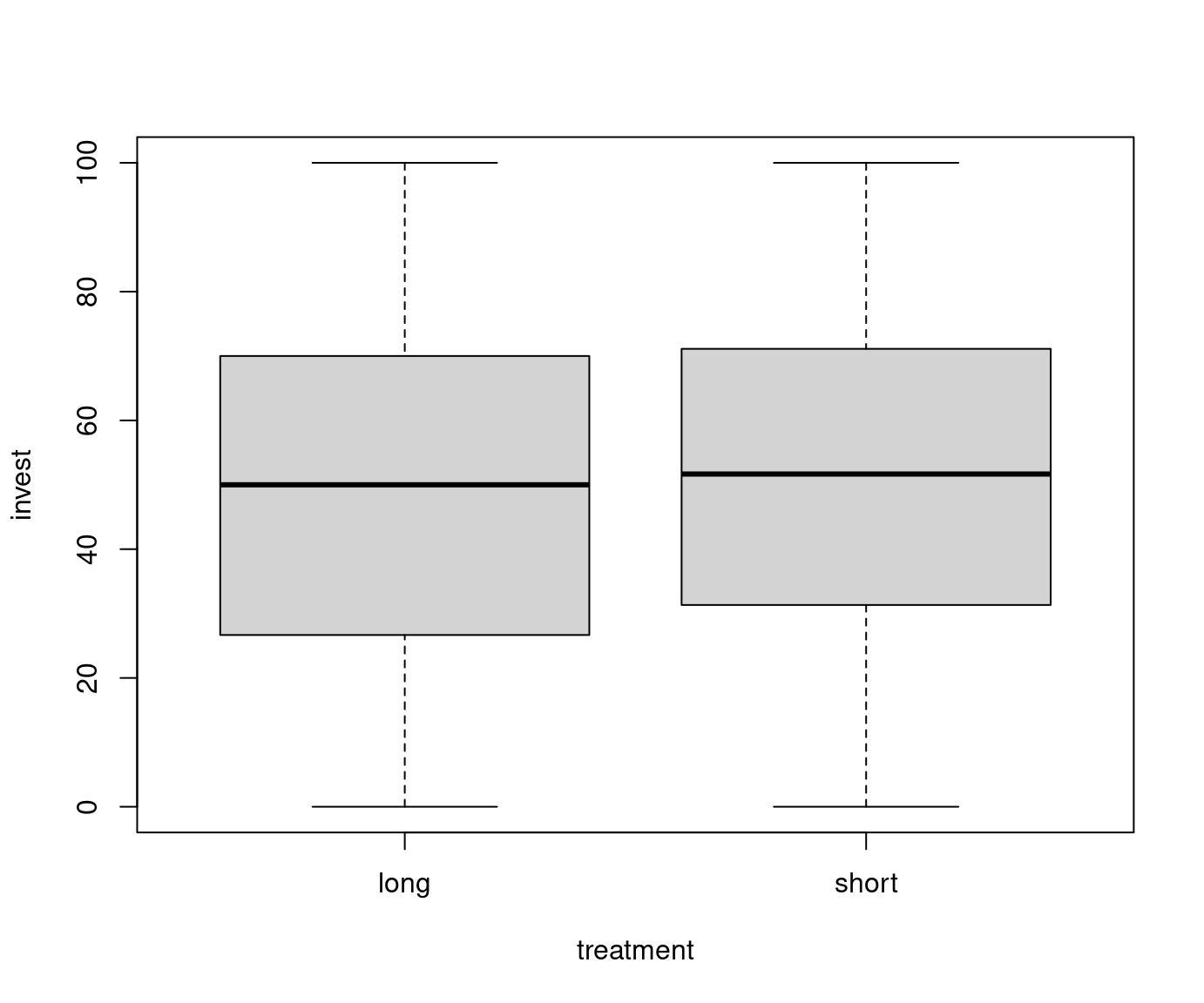
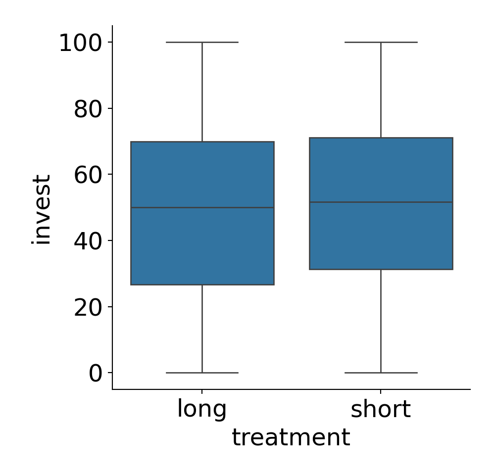
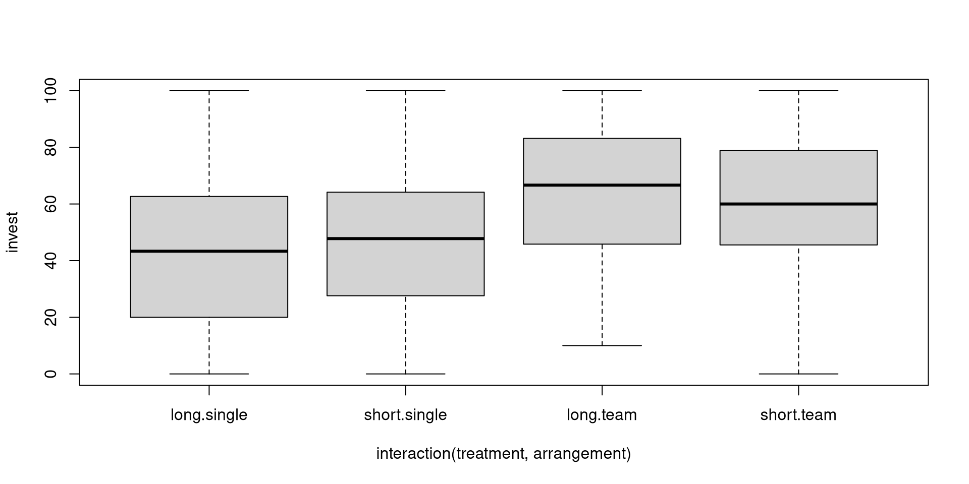
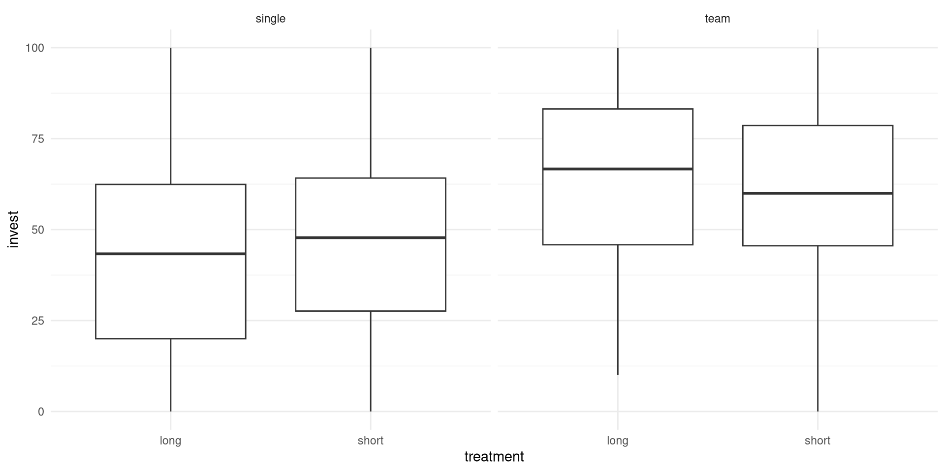
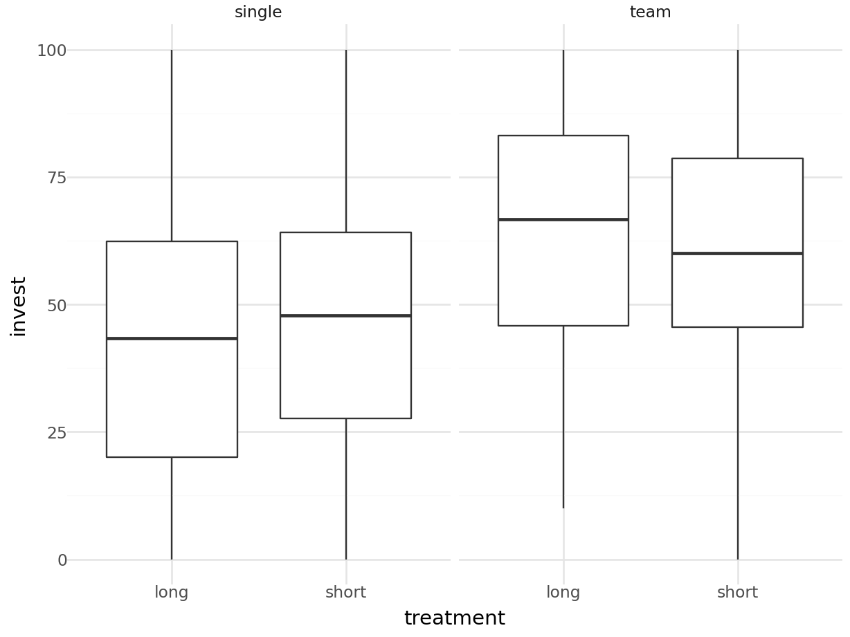
Example: Dependence of investments on both arrangement (single vs. team) and the main treatment (long vs. short).
Data:
##     invest arrangement treatment
## 1    70.00        team      long
## 8    60.00        team      long
## 159  56.67        team     short
## 310  52.67      single      long
## ...Univariate statistics:
##      invest      arrangement  treatment
##  Min.   :  0.0   single:385   long :285
##  1st Qu.: 30.0   team  :185   short:285
##  Median : 50.0
##  Mean   : 50.4
##  3rd Qu.: 70.0
##  Max.   :100.0
14.2.1 Visualization

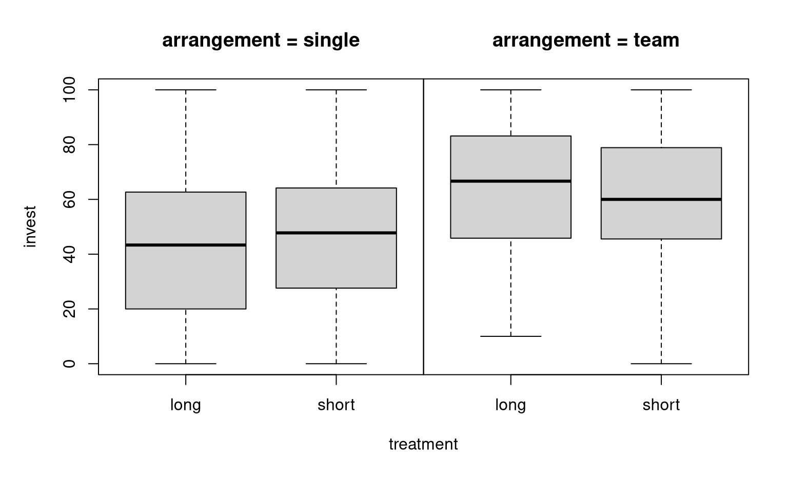
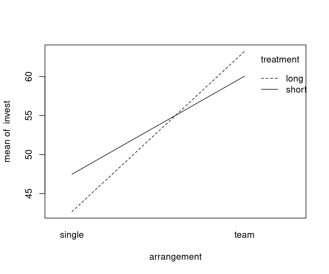
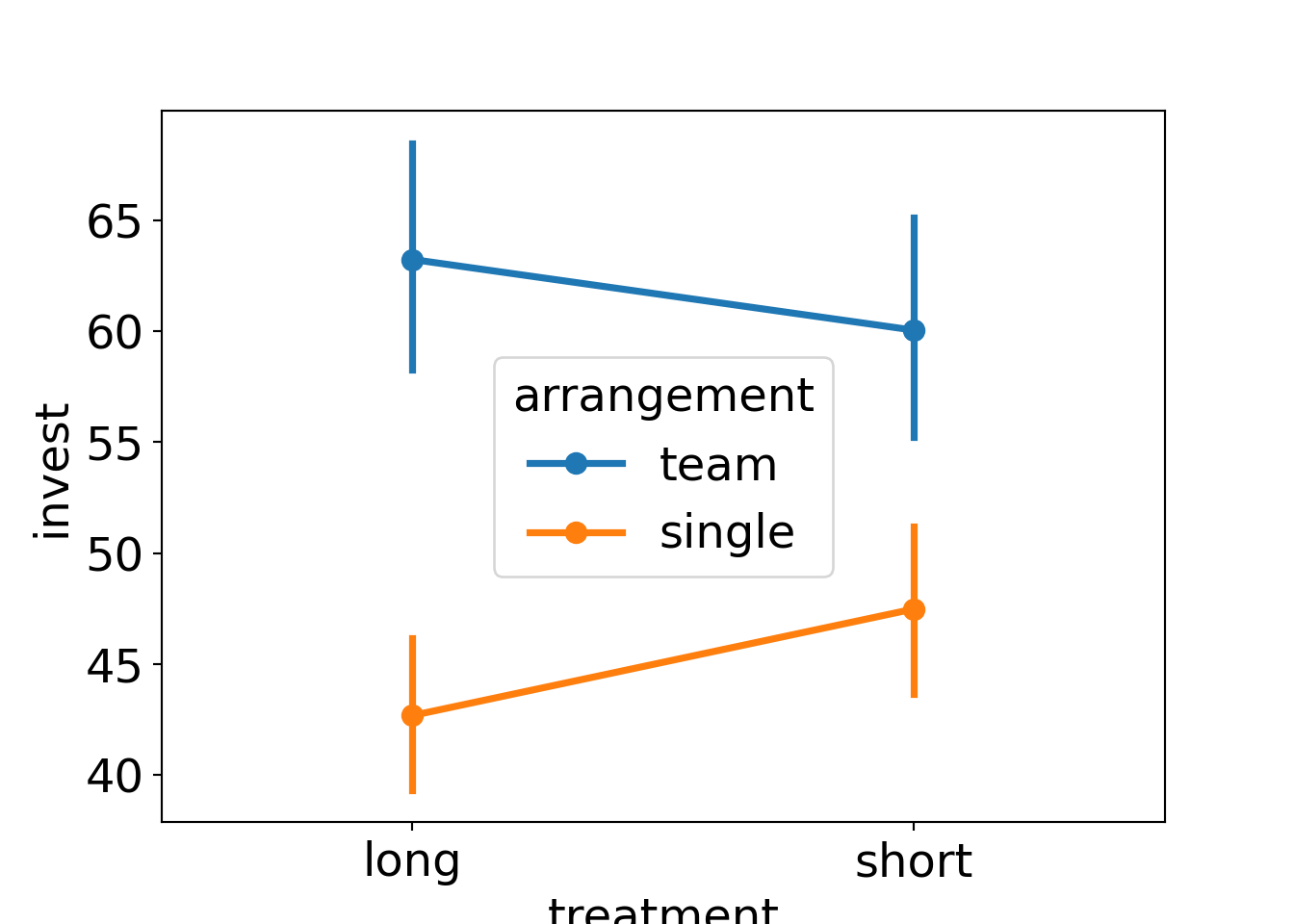
Groupwise statistics:
| Long | Short | ||
|---|---|---|---|
| Single | \(\overline y\) | 42.68 | 47.48 |
| \(n\) | 198 | 187 | |
| \(s\) | 25.33 | 27.02 | |
| Team | \(\overline y\) | 63.23 | 60.05 |
| \(n\) | 87 | 98 | |
| \(s\) | 24.05 | 24.91 |
Observations:
- There is a clear
arrangementeffect. - The
treatmenteffect is very small. - For teams, investments in the short (compared to long) treatment are somewhat smaller (compatible with the myopia hypothesis)
- For single players, the short effect is even smaller and slightly positive.
Questions:
- Are the
arrangementand/ortreatmenteffects significant? - Is there a significant interaction effect?
- How can the effects be coded in a linear model?
- Which of the possible models should be selected?
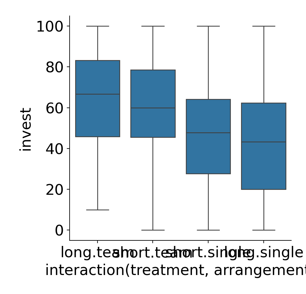
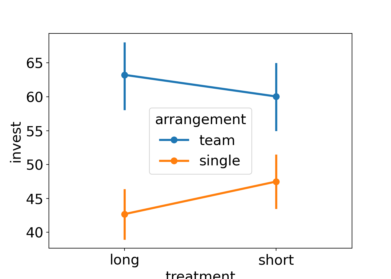
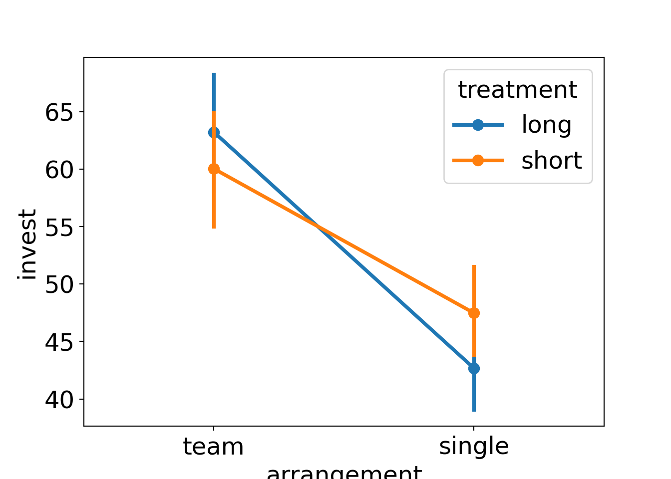
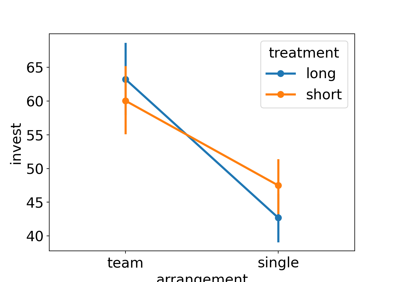
Additional visualization: Interaction plot for group means.
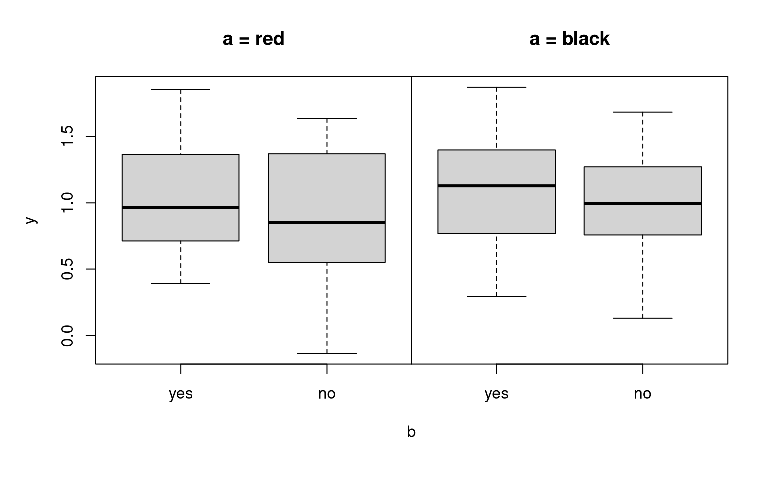
14.2.3 Artificial example: 2-way Analysis of Variance
Artificial example:
Model the expectation of y using two factors:
a with levels black and red,
b with levels yes and no.
Thus: Four possible subsamples with corresponding expectations of y.
a vs. b |
yes | no |
|---|---|---|
| red | \(\mu_{\mathsf{red}, \mathsf{yes}}\) | \(\mu_{\mathsf{red}, \mathsf{no}}\) |
| black | \(\mu_{\mathsf{black}, \mathsf{yes}}\) | \(\mu_{\mathsf{black}, \mathsf{no}}\) |
Question: How does the expectation \(\mu\) of y depend on the variables a and b?
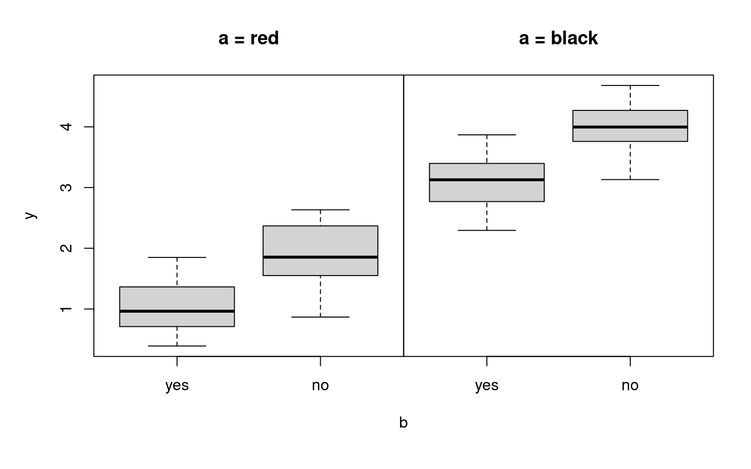
Trivial: If all expectations are equal
\[ \mu_{\mathsf{red}, \mathsf{yes}} = \dots = \mu_{\mathsf{black}, \mathsf{no}} \]
y depends neither on a nor b. The constant expectation
can be estimated from the pooled sample using the overall mean.
In R: lm(y ~ 1)
Example:
a vs. b |
yes | no |
|---|---|---|
| red | \(2\) | \(2\) |
| black | \(2\) | \(2\) |

##
## Call:
## lm(formula = y ~ 1, data = dat)
##
## Residuals:
## Min 1Q Median 3Q Max
## -1.1382 -0.3668 0.0116 0.3641 0.8622
##
## Coefficients:
## Estimate Std. Error t value Pr(>|t|)
## (Intercept) 2.0055 0.0428 46.9 <2e-16
##
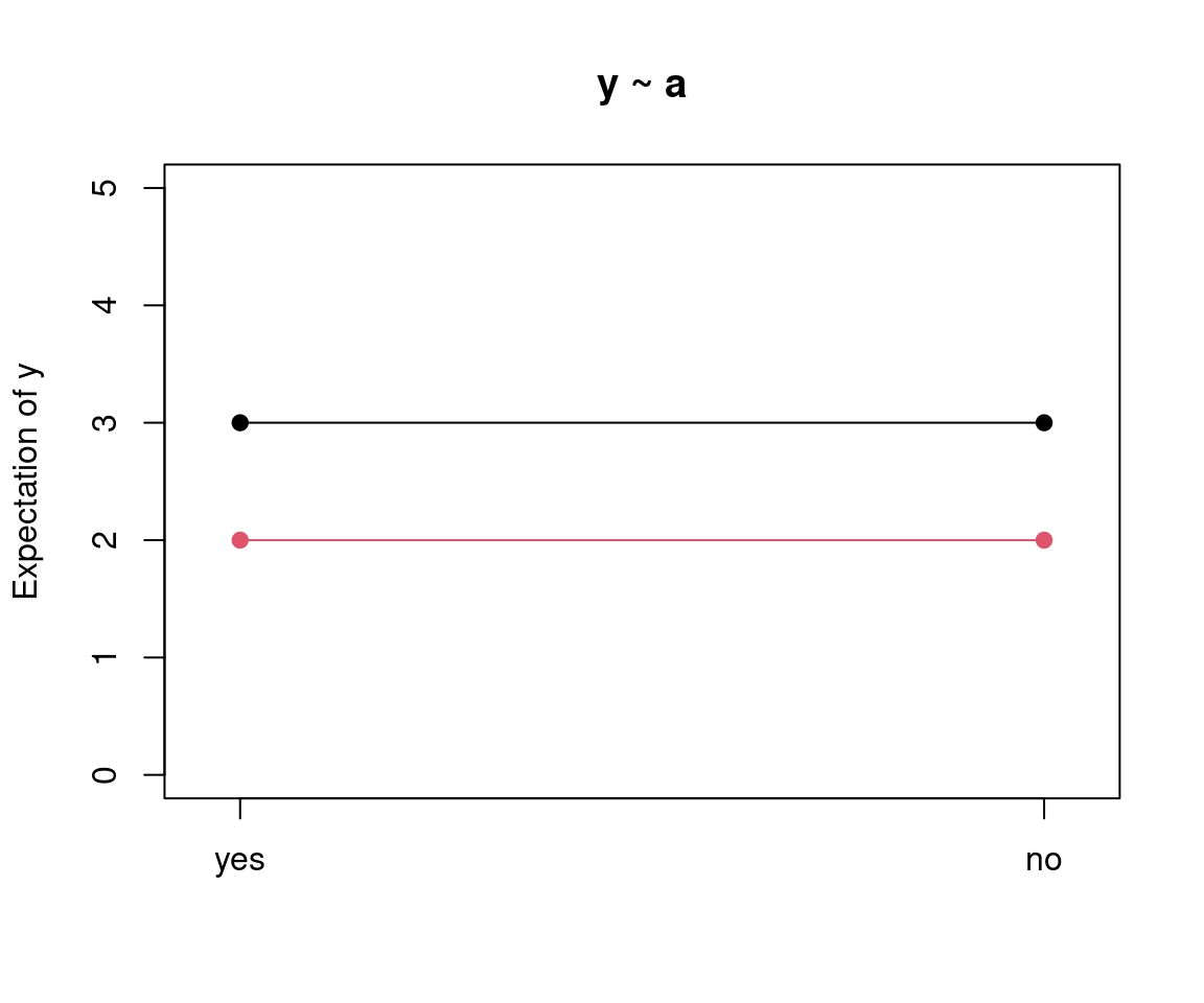
## Residual standard error: 0.428 on 99 degrees of freedomAlso clear: If only a but not b has an effect on y, then the rows in the expectation matrix differ but not the columns.
In R: lm(y ~ a)
Example:
a vs. b |
yes | no |
|---|---|---|
| red | \(2\) | \(2\) |
| black | \(3\) | \(3\) |

##
## Call:
## lm(formula = y ~ a, data = dat)
##
## Residuals:
## Min 1Q Median 3Q Max
## -1.1007 -0.3390 0.0486 0.3875 0.8814
##
## Coefficients:
## Estimate Std. Error t value Pr(>|t|)
## (Intercept) 1.9680 0.0606 32.5 <2e-16
## ablack 1.0750 0.0857 12.5 <2e-16
##
## Residual standard error: 0.429 on 98 degrees of freedom
## Multiple R-squared: 0.616, Adjusted R-squared: 0.612
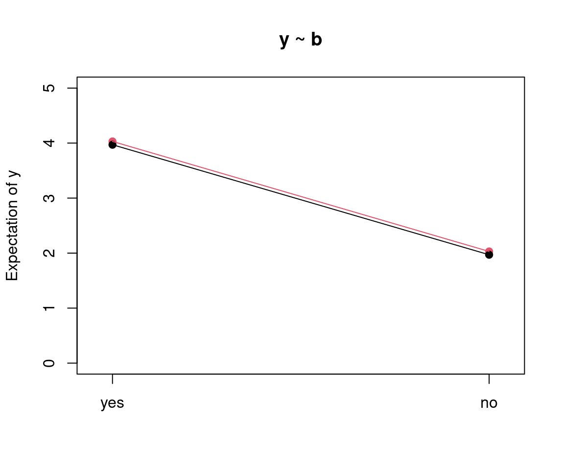
## F-statistic: 157 on 1 and 98 DF, p-value: <2e-16Analogously: If only b but not a has an effect on y, then the columns in the expectation matrix differ but not the rows.
In R: lm(y ~ b)
Example:
a vs. b |
yes | no |
|---|---|---|
| red | \(4\) | \(2\) |
| black | \(4\) | \(2\) |

##
## Call:
## lm(formula = y ~ b, data = dat)
##
## Residuals:
##     Min      1Q  Median      3Q     Max
## -1.0975 -0.3586  0.0309  0.3602  0.8215
##
## Coefficients:
##             Estimate Std. Error t value Pr(>|t|)
## (Intercept)   4.0462     0.0606    66.8   <2e-16
## bno          -2.0814     0.0856   -24.3   <2e-16
##
## Residual standard error: 0.428 on 98 degrees of freedom
## Multiple R-squared:  0.858,  Adjusted R-squared:  0.856
## F-statistic:  591 on 1 and 98 DF,  p-value: <2e-16
Two main effects: Just like for quantitative explanatory variables, several additive effects for indicator variables from qualitative explanatory variables can be considered.
In R: lm(y ~ a + b)
Interpretation: There is a black effect and a no effect. Both effects are additive. Thus, the black effect does not depend on the level of b (yes vs. no). Conversely, the no effect does not depend on the level of a (black vs. red).
Example:
a vs. b |
yes | no |
|---|---|---|
| red | \(1\) | \(2\) |
| black | \(3\) | \(4\) |
##
## Call:
## lm(formula = y ~ a + b, data = dat)
##
## Residuals:
## Min 1Q Median 3Q Max
## -1.060 -0.335 0.029 0.372 0.841
##
## Coefficients:
## Estimate Std. Error t value Pr(>|t|)
## (Intercept) 1.0087 0.0743 13.6 <2e-16
## ablack 2.0750 0.0858 24.2 <2e-16
## bno 0.9186 0.0858 10.7 <2e-16
##
## Residual standard error: 0.429 on 97 degrees of freedom
## Multiple R-squared: 0.878, Adjusted R-squared: 0.876
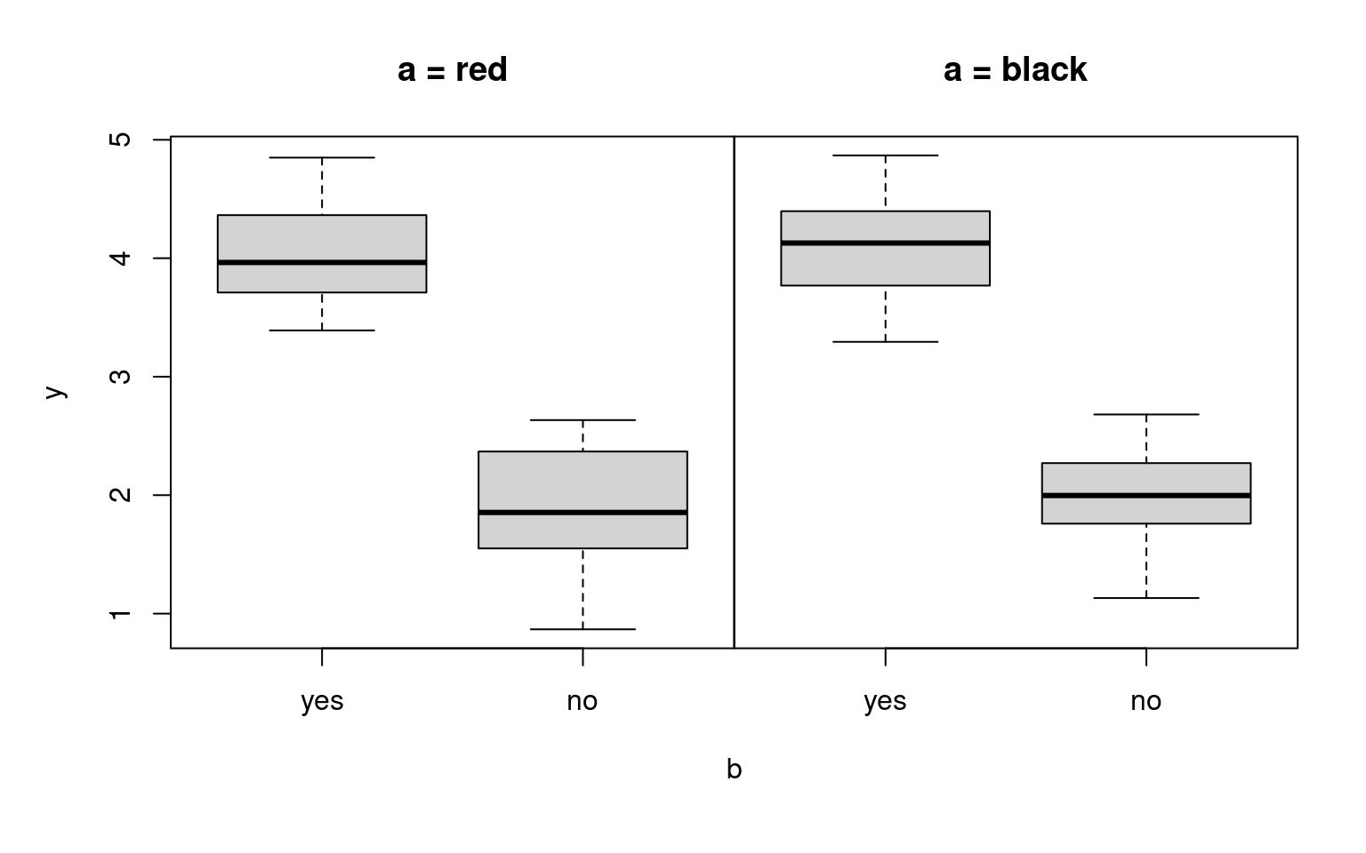
## F-statistic: 350 on 2 and 97 DF, p-value: <2e-16Interaction effect: If the black effect and the no effect interact, then the no effect depends on whether a falls into category black or red. Conversely, the black effect depends on whether b falls into category yes or no.
In R: lm(y ~ a + b + a:b)
Jargon: The effects a and b are called main effects and a:b is the interaction effect. A short notation combining both is: lm(y ~ a * b)
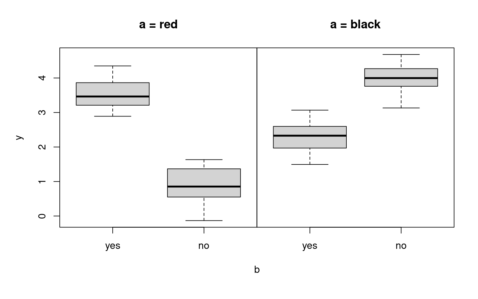
Example:
a vs. b |
yes | no |
|---|---|---|
| red | \(3.5\) | \(1.0\) |
| black | \(2.2\) | \(4.0\) |


##
## Call:
## lm(formula = y ~ a * b, data = dat)
##
## Residuals:
##     Min      1Q  Median      3Q     Max
## -1.0496 -0.3273  0.0299  0.3644  0.8303
##
## Coefficients:
##             Estimate Std. Error t value Pr(>|t|)
## (Intercept)   3.5191     0.0862    40.8   <2e-16
## ablack       -1.2458     0.1219   -10.2   <2e-16
## bno          -2.6022     0.1219   -21.4   <2e-16
## ablack:bno    4.3415     0.1723    25.2   <2e-16
##
## Residual standard error: 0.431 on 96 degrees of freedom
## Multiple R-squared:  0.89,   Adjusted R-squared:  0.886
## F-statistic:  258 on 3 and 96 DF,  p-value: <2e-16
Remark: The maximal number of \(2 \cdot 2 = 4\) parameters is estimated in the interaction model
y ~ a + b + a:b
Question: How is the interaction effect coded in this model?
Clear: The first coefficient is the intercept which corresponds to the red and yes group. a and b are transformed to indicator variables for black and no, respectively.
Answer: If both effects are observed simultaneously (i.e., black and no), then there is an additional coefficient, corresponding to the interaction effect. The corresponding indicator variable is simply the product of the black and no indicator variables.
Matrix notation:
\[\begin{equation*} \left( \begin{array}{c} y_1 \\ y_2 \\ y_3 \\ y_4 \\ y_5 \\ \vdots \\ \end{array} \right) \quad = \quad \left(\begin{array}{cccc} 1 & 0 & 0 & 0 \\ 1 & 1 & 0 & 0 \\ 1 & 0 & 1 & 0 \\ 1 & 1 & 1 & 1 \\ 1 & 1 & 0 & 0 \\ & {\vdots} & \end{array} \right) ~ \left( \begin{array}{l} \beta_1 \\ \beta_\mathtt{ablack} \\ \beta_\mathtt{bno} \\ \beta_\mathtt{ablack:bno} \\ \end{array} \right) ~+~ \left( \begin{array}{c} \varepsilon_1 \\ \varepsilon_2 \\ \varepsilon_3 \\ \varepsilon_4 \\ \varepsilon_5 \\ \vdots \ \end{array} \right) \end{equation*}\]
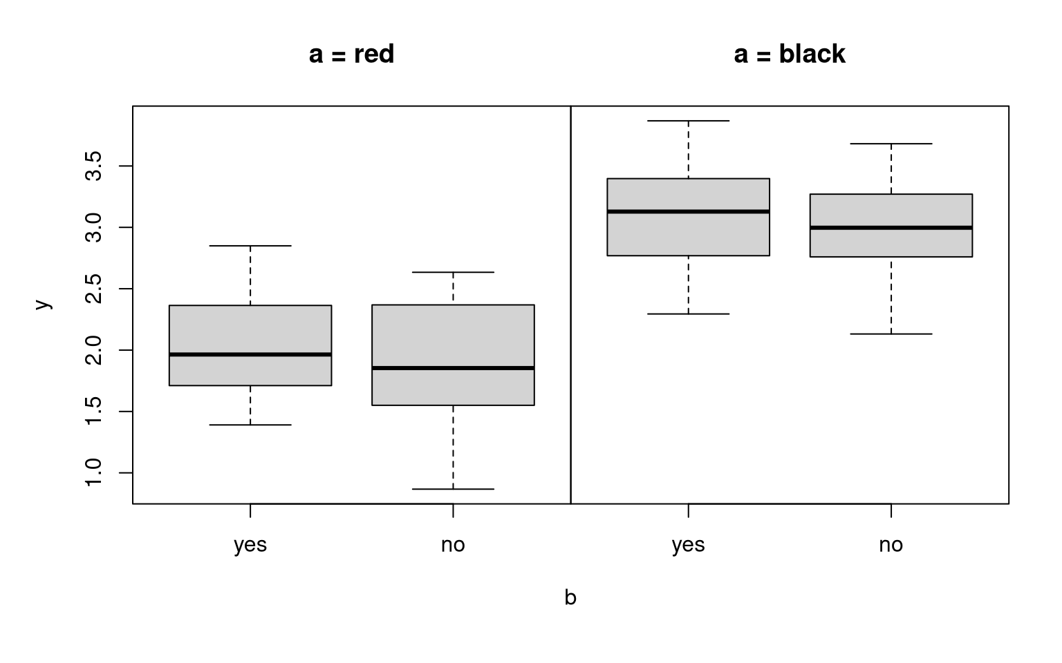
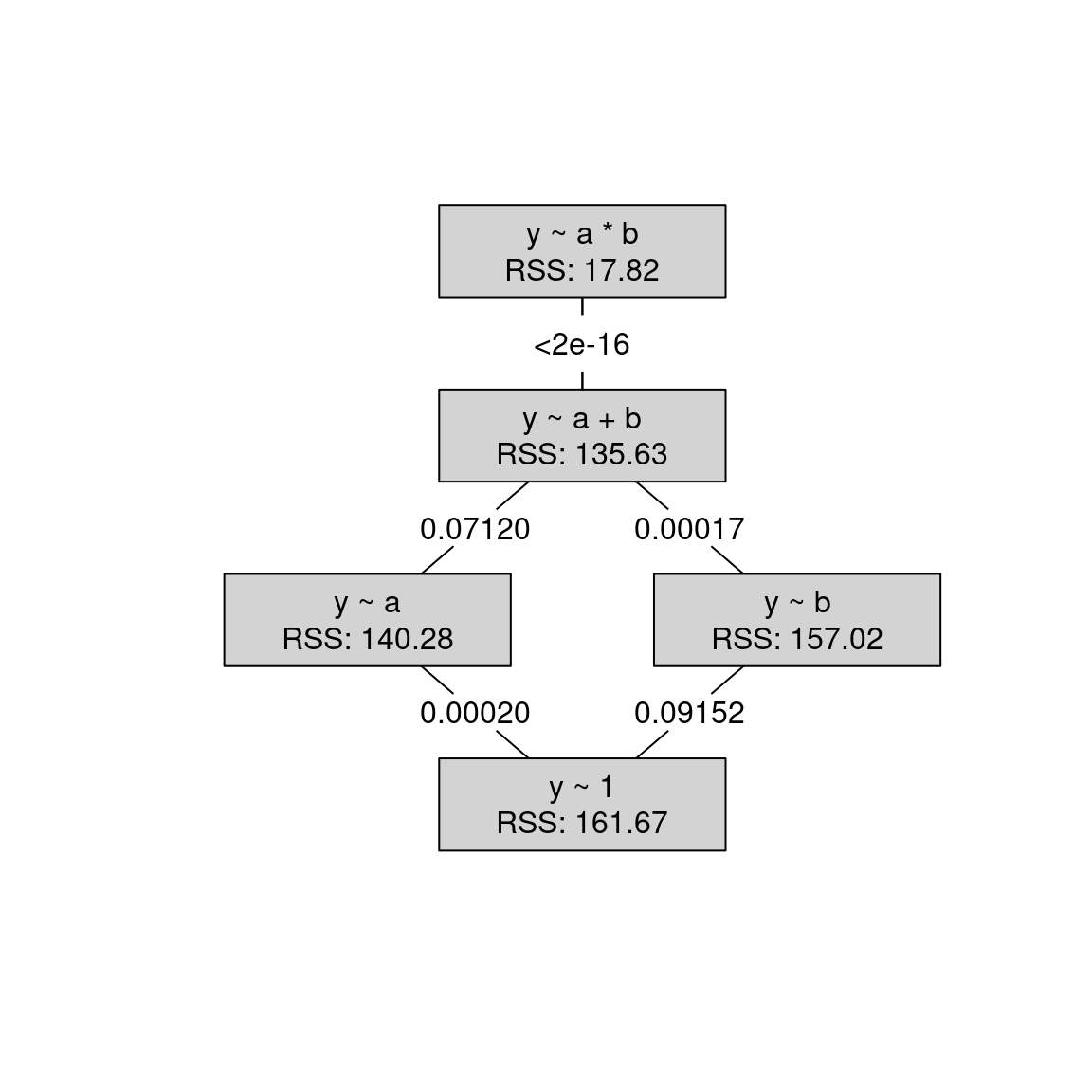
14.2.4 Model selection: 2-way Analysis of Variance
Question: Which of the possible models should be selected for a given data set?
Answer: Model selection “as usual” in linear models, e.g., based on \(F\)-tests.
Attention: The interpretation of the interaction effect is only straightforward if both corresponding main effects are also included in the model. Thus, it is possible to fit a model like the following but almost never meaningful:
y ~ a + a:b
Thus: In a backward selection test the interaction effect first. Only in the case of non-significance proceed to test the main effects.
Example: Artificial data for the true y ~ a * b and y ~ 1 models, respectively.

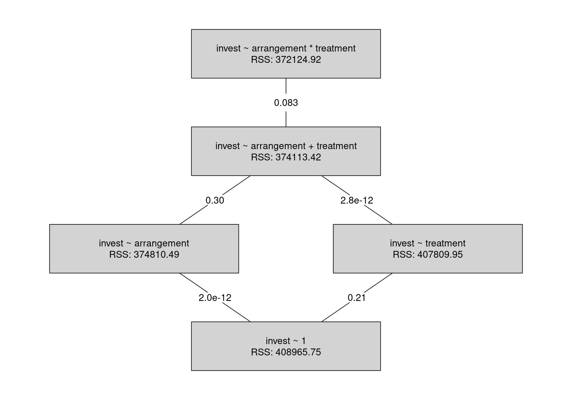

14.2.5 MLA: 2-way Analysis of Variance
Example: Investments in the myopic loss aversion experiment, depending on arrangement (single vs. team) and treatment (long vs. short).
Interpretation:
- The interaction effect is not significant at 5% level (\(p = 0.083\)).
- The model can be simplified by first omitting the interaction effect and then the treatment main effect.
- Only the arrangement effect (already discussed above) remains.
Remark: The significance of the interaction effect decreases further when incorporating other relevant explanatory variables into the model. See below.

##
## Call:
## lm(formula = invest ~ arrangement * treatment, data = MLA)
##
## Residuals:
##    Min     1Q Median     3Q    Max
## -60.05 -20.62   0.65  17.63  57.32
##
## Coefficients:
##                                Estimate Std. Error t value     Pr(>|t|)
## (Intercept)                       42.68       1.82   23.42      < 2e-16
## arrangementteam                   20.55       3.30    6.23 0.0000000009
## treatmentshort                     4.80       2.61    1.84        0.067
## arrangementteam:treatmentshort    -7.99       4.59   -1.74        0.083
##
## Residual standard error: 25.6 on 566 degrees of freedom
## Multiple R-squared:  0.0901, Adjusted R-squared:  0.0853
## F-statistic: 18.7 on 3 and 566 DF,  p-value: 0.0000000000145
14.3 Tutorial
The myopic loss aversion (MLA) data (MLA.csv, MLA.rda) already analyzed in Chapter 13 are reconsidered. Here, the dependence of invested point percentages
(invest) on up to two explanatory variables and their interaction term is considered.
Chapter 16 will consider all available explanatory variables along with potential interactions.
14.3.1 Setup
Python
# Make sure that the required libraries are installed.
# Import the necessary libraries and classes:
import pandas as pd
import numpy as np
import matplotlib.pyplot as plt
import seaborn as sns
import statsmodels.api as sm
import statsmodels.formula.api as smf

pd.set_option("display.precision", 4) # Set display precision to 4 digits in pandas and numpy.
# Load dataset
MLA = pd.read_csv("MLA.csv", index_col=False, header=0)
# Preview the first 5 lines of the loaded data
MLA.head(5)## invest gender male age treatment grade arrangement
## 0 70.0000 female/male yes 11.7533 long 6-8 team
## 1 28.3333 female/male yes 12.0866 long 6-8 team
## 2 50.0000 female/male yes 11.7950 long 6-8 team
## 3 50.0000 male yes 13.7566 long 6-8 team
## 4 24.3333 female/male yes 11.2950 long 6-8 team14.3.2 1-way analysis of variance
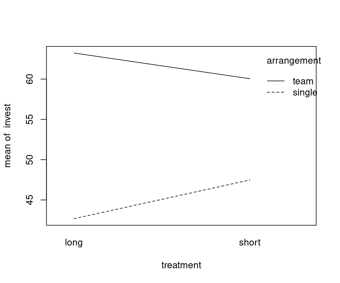
Plot invest against arrangement:

Linear model: invest explained by arrangement:
R
##
## Call:
## lm(formula = invest ~ arrangement, data = MLA)
##
## Residuals:
##    Min     1Q Median     3Q    Max
## -61.55 -19.77  -0.01  18.32  54.99
##
## Coefficients:
##                 Estimate Std. Error t value Pr(>|t|)
## (Intercept)        45.01       1.31   34.38   <2e-16
## arrangementteam    16.53       2.30    7.19    2e-12
##
## Residual standard error: 25.7 on 568 degrees of freedom
## Multiple R-squared:  0.0835, Adjusted R-squared:  0.0819
## F-statistic: 51.8 on 1 and 568 DF,  p-value: 1.99e-12
Python
##                             OLS Regression Results
## ==============================================================================
## Dep. Variable:                 invest   R-squared:                       0.084
## Model:                            OLS   Adj. R-squared:                  0.082
## Method:                 Least Squares   F-statistic:                     51.76
## Date:                Wed, 05 Mar 2025   Prob (F-statistic):           1.99e-12
## Time:                        14:23:21   Log-Likelihood:                -2658.0
## No. Observations:                 570   AIC:                             5320.
## Df Residuals:                     568   BIC:                             5329.
## Df Model:                           1
## Covariance Type:            nonrobust
## =======================================================================================
##                           coef    std err          t      P>|t|      [0.025      0.975]
## ---------------------------------------------------------------------------------------
## Intercept              45.0124      1.309     34.382      0.000      42.441      47.584
## arrangement[T.team]    16.5329      2.298      7.194      0.000      12.019      21.047
## ==============================================================================
## Omnibus:                       33.822   Durbin-Watson:                   1.514
## Prob(Omnibus):                  0.000   Jarque-Bera (JB):               14.624
## Skew:                           0.148   Prob(JB):                     0.000667
## Kurtosis:                       2.274   Cond. No.                         2.41
## ==============================================================================
##
## Notes:
## [1] Standard Errors assume that the covariance matrix of the errors is correctly specified.
Fit the main effects model of all explanatory variables for modeling invest in the MLA data, and analysis of variance:
Plot invest against gender:
Linear model: invest ~ gender and analysis of variance:
Summary of the linear model invest ~ gender
R
##
## Call:
## lm(formula = invest ~ gender, data = MLA)
##
## Residuals:
##    Min     1Q Median     3Q    Max
## -65.37 -20.34   0.08  19.77  56.43
##
## Coefficients:
##                   Estimate Std. Error t value Pr(>|t|)
## (Intercept)          43.57       1.43   30.51   <2e-16
## genderfemale/male    21.80       3.10    7.03    6e-12
## gendermale           12.24       2.45    4.99    8e-07
##
## Residual standard error: 25.5 on 567 degrees of freedom
## Multiple R-squared:  0.0954, Adjusted R-squared:  0.0922
## F-statistic: 29.9 on 2 and 567 DF,  p-value: 4.51e-13
Python
##                             OLS Regression Results
## ==============================================================================
## Dep. Variable:                 invest   R-squared:                       0.095
## Model:                            OLS   Adj. R-squared:                  0.092
## Method:                 Least Squares   F-statistic:                     29.90
## Date:                Wed, 05 Mar 2025   Prob (F-statistic):           4.51e-13
## Time:                        14:23:23   Log-Likelihood:                -2654.3
## No. Observations:                 570   AIC:                             5315.
## Df Residuals:                     567   BIC:                             5328.
## Df Model:                           2
## Covariance Type:            nonrobust
## =========================================================================================
##                             coef    std err          t      P>|t|      [0.025      0.975]
## -----------------------------------------------------------------------------------------
## Intercept                43.5656      1.428     30.510      0.000      40.761      46.370
## gender[T.female/male]    21.8039      3.103      7.028      0.000      15.710      27.898
## gender[T.male]           12.2447      2.453      4.992      0.000       7.427      17.063
## ==============================================================================
## Omnibus:                       41.371   Durbin-Watson:                   1.581
## Prob(Omnibus):                  0.000   Jarque-Bera (JB):               14.658
## Skew:                           0.033   Prob(JB):                     0.000656
## Kurtosis:                       2.217   Cond. No.                         3.33
## ==============================================================================
##
## Notes:
## [1] Standard Errors assume that the covariance matrix of the errors is correctly specified.
14.3.3 2-way analysis of variance
Base graphics:


Interaction between treatment and arrangement:
lattice graphics (available in R):
ggplot2 graphics:
length and sd instead of mean.
Analysis of variance:
R
## Analysis of Variance Table
##
## Model 1: invest ~ 1
## Model 2: invest ~ arrangement
## Model 3: invest ~ arrangement + treatment
## Model 4: invest ~ arrangement * treatment
##   Res.Df    RSS Df Sum of Sq     F  Pr(>F)
## 1    569 408966
## 2    568 374810  1     34155 51.95 1.8e-12
## 3    567 374113  1       697  1.06   0.304
## 4 566 372125 1 1988 3.02 0.083## Analysis of Variance Table
##
## Model 1: invest ~ 1
## Model 2: invest ~ treatment
## Model 3: invest ~ arrangement + treatment
## Model 4: invest ~ arrangement * treatment
## Res.Df RSS Df Sum of Sq F Pr(>F)
## 1 569 408966
## 2 568 407810 1 1156 1.76 0.185
## 3 567 374113 1 33697 51.25 2.5e-12
## 4 566 372125 1 1988 3.02 0.083Python
##    df_resid          ssr  df_diff     ss_diff        F      Pr(>F)
## 0     569.0  408965.7464      0.0         NaN      NaN         NaN
## 1     568.0  374810.4899      1.0  34155.2565  51.9500  1.8224e-12
## 2     567.0  374113.4219      1.0    697.0680   1.0602  3.0360e-01
## 3 566.0 372124.9236 1.0 1988.4983 3.0245 8.2560e-02## df_resid ssr df_diff ss_diff F Pr(>F)
## 0 569.0 408965.7464 0.0 NaN NaN NaN
## 1 568.0 407809.9516 1.0 1155.7948 1.7580 1.8541e-01
## 2 567.0 374113.4219 1.0 33696.5297 51.2522 2.5289e-12
## 3 566.0 372124.9236 1.0 1988.4983 3.0245 8.2560e-02Summary of invest ~ arrangement:
R
##
## Call:
## lm(formula = invest ~ arrangement, data = MLA)
##
## Residuals:
##    Min     1Q Median     3Q    Max
## -61.55 -19.77  -0.01  18.32  54.99
##
## Coefficients:
##                 Estimate Std. Error t value Pr(>|t|)
## (Intercept)        45.01       1.31   34.38   <2e-16
## arrangementteam    16.53       2.30    7.19    2e-12
##
## Residual standard error: 25.7 on 568 degrees of freedom
## Multiple R-squared:  0.0835, Adjusted R-squared:  0.0819
## F-statistic: 51.8 on 1 and 568 DF,  p-value: 1.99e-12
Python
##                             OLS Regression Results
## ==============================================================================
## Dep. Variable:                 invest   R-squared:                       0.084
## Model:                            OLS   Adj. R-squared:                  0.082
## Method:                 Least Squares   F-statistic:                     51.76
## Date:                Wed, 05 Mar 2025   Prob (F-statistic):           1.99e-12
## Time:                        14:23:30   Log-Likelihood:                -2658.0
## No. Observations:                 570   AIC:                             5320.
## Df Residuals:                     568   BIC:                             5329.
## Df Model:                           1
## Covariance Type:            nonrobust
## =======================================================================================
##                           coef    std err          t      P>|t|      [0.025      0.975]
## ---------------------------------------------------------------------------------------
## Intercept              45.0124      1.309     34.382      0.000      42.441      47.584
## arrangement[T.team]    16.5329      2.298      7.194      0.000      12.019      21.047
## ==============================================================================
## Omnibus:                       33.822   Durbin-Watson:                   1.514
## Prob(Omnibus):                  0.000   Jarque-Bera (JB):               14.624
## Skew:                           0.148   Prob(JB):                     0.000667
## Kurtosis:                       2.274   Cond. No.                         2.41
## ==============================================================================
##
## Notes:
## [1] Standard Errors assume that the covariance matrix of the errors is correctly specified.