Chapter 7 Hierarchical clustering
7.1 Cluster analysis
Idea: Obtain a classification of objects (observations) into groups (clusters) so that distances within the groups are small but distances between groups are large.
Goals:
- Homogeneity within the clusters.
- Heterogeneity between the clusters.
Still needed: Suitable distance measures within/between clusters for assessing homogeneity/heterogeneity.
Here: The classifications considered are either partitions or hierarchies of partitions.
Definition: A partition is a segmentation of \(n\) objects into \(k\) clusters so that each object belongs to exactly one cluster.
Thus: The union of all clusters yields the entire population while the pairwise intersections are empty.
Formally: A partition \(\mathcal{C}\) is a set of \(k\) clusters
\[ \mathcal{C} \quad = \quad \{C_1, \dots, C_k\} \]
where each cluster \(C_j\) is a set of objects so that
\[\begin{eqnarray*} C_1 \; \cup \; \dots \; \cup \; C_k & = & \{x_1, \dots, x_n\} \\ C_i \; \cap \; C_j & = & \emptyset \end{eqnarray*}\]
Moreover: A hierarchy of partitions is a sequence of partitions \(\mathcal{C}_1, \mathcal{C}_2, \dots\) where each \(\mathcal{C}_j\) and subsequent \(\mathcal{C}_{j+1}\) only differ in (at least) one cluster from \(\mathcal{C}_j\) being partitioned once more.
7.2 Distances
Previously: In scatter plots and biplots we have always considered distances between the points in the plots.
- Points/observations that are close in the plot are interpreted to be similar.
- Points/observations that are distant are dissimilar.
Excursion: How to judge distances/dissimilarities between two observations/rows of data matrix \(X\) more generally?
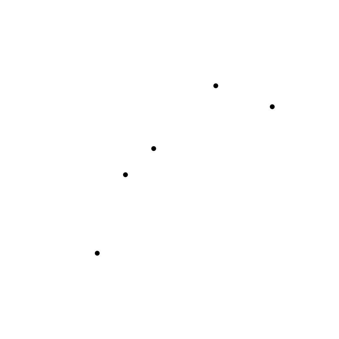
Example: Distance between two points \(x_1 = (2, 1)\) and \(x_2 = (5, 5)\).
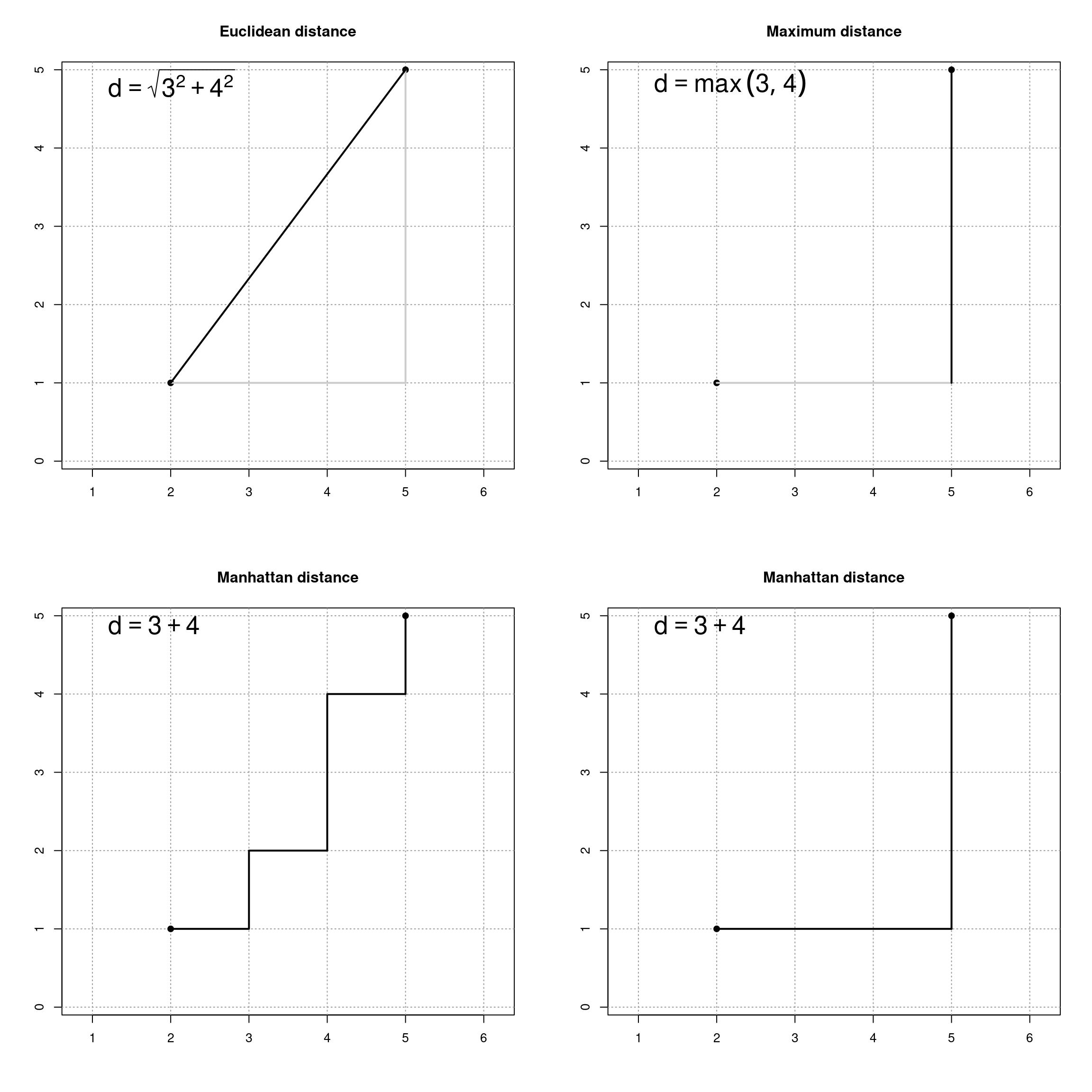
Formally: Let \(x_1\) and \(x_2\) be two different observations/rows from \(X\).
Manhattan distance: \[ d_1(x_1, x_2) \quad = \quad \sum_{j = 1}^p | x_{1j} - x_{2j} | \]
Euclidean distance: \[ d_2(x_1, x_2) \quad = \quad \sqrt{ \sum_{j = 1}^p (x_{1j} - x_{2j})^2 }\] Maximum distance: \[ d_\infty(x_1, x_2) \quad = \quad \max_{j = 1, \dots, p} | x_{1j} - x_{2j} | \]
Canberra distance: \[ d_\mathsf{C}(x_1, x_2) \quad = \quad \sum_{j = 1}^p \frac{| x_{1j} - x_{2j} |}{| x_{1j} | + | x_{2j} |} \]
Additionally: Special distances for binary variables.
Idea: Two “successes” (\(x_{1j} = x_{2j} = 1\)) have more common, i.e., are closer, than two “failures” (\(x_{1j} = x_{2j} = 0\)).
Popular solution: Use the proportion of variables per observation that are discordant among those where at least one is a “success”.
- First omit all variables/columns where both observations are \(0\).
- Compute proportion of discordant columns, i.e., where one observation is \(0\) and the other \(1\).
Jargon: This distance is also known as asymmetric binary or Jaccard or Tanimoto distance.
7.3 Distances between clusters
Question: How to define distances between clusters (sets of observations) rather than individual observations?
Solution: Define a distance measure \(D(\cdot, \cdot)\) for clusters based on the distance measure \(d(\cdot, \cdot)\), obtained for all pairs of observations.
Thus: All the distance measures defined above (for observations) can be used as the basis for a distance measure between clusters.
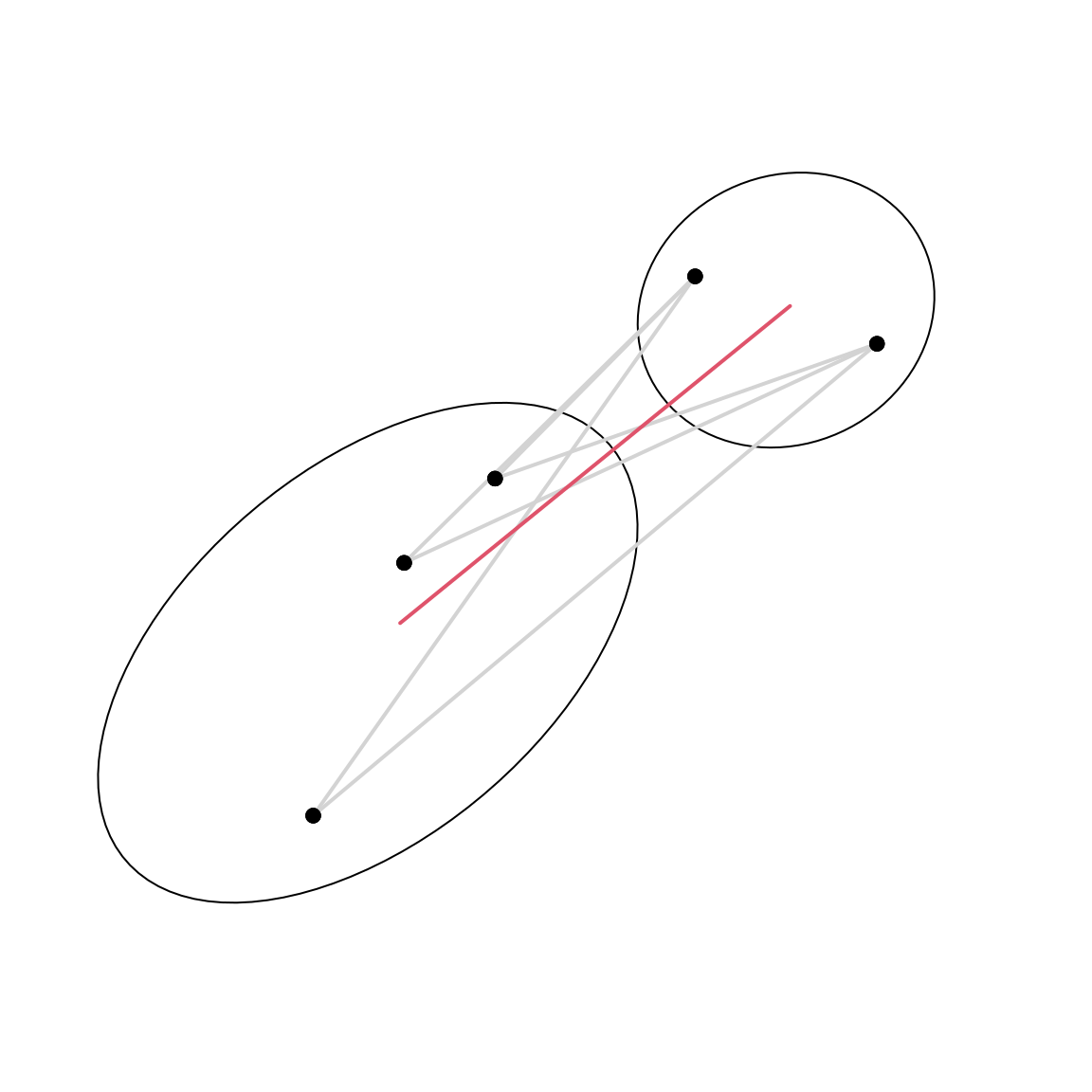
Idea 1: Define the distance between two clusters as the distance between the two most similar objects from these clusters.
\[ D_\mathsf{s}(C_1, C_2) \quad = \quad \min_{x \in C_1, y \in C_2} d(x, y) \] Jargon: Cluster analyses based on this heterogeneity measure are also called single linkage or nearest neighbour methods.
Problem: Tends to underestimate heterogeneity.
Idea 2: Define the distance between two clusters as the distance between the two most dissimilar objects from these clusters.
\[ D_\mathsf{c}(C_1, C_2) \quad = \quad \max_{x \in C_1, y \in C_2} d(x, y) \] Jargon: Cluster analyses based on this heterogeneity measure are also called complete linkage or distant neighbour methods.
Problem: Tends to overestimate heterogeneity.
Idea 3: Define the distance between two clusters as the average distance between all pairs of objects.
\[ D_\mathsf{a}(C_1, C_2) \quad = \quad \frac{1}{|C_1||C_2|} \sum_{x \in C_1} \sum_{y \in C_2} d(x, y) \]
Jargon: Cluster analyses based on this heterogeneity measure are also called average linkage.
Distances between clusters: Single

Distances between clusters: Complete
Distances between clusters: Average
Furthermore: Ward method.
Idea: A type of analysis of variance, comparing the error sum of squares within two clusters with the error sum of squares within the union of these clusters.
\[\begin{eqnarray*} D_w(C_1 \cup C_2, C_3) & = & \frac{|C_1| + |C_3|}{|C_1| + |C_2| + |C_3|} D_w(C_1, C_3) + \\ & & \frac{|C_2| + |C_3|}{|C_1| + |C_2| + |C_3|} D_w(C_2, C_3) - \\ & & \frac{|C_1| + |C_2|}{|C_1| + |C_2| + |C_3|} D_w(C_1, C_2) \end{eqnarray*}\]
Initialization: Squared (or sometimes also absolute) distances between the individual observations (i.e., clusters with just one observation each).
Analogously: Define measures for homogeneity within clusters based on distances between pairs of observations from the same cluster.
- Maximum distance.
- Minimum distance.
- Average distance.
7.4 Hierarchical clustering
Idea: Cluster methods that generate hierarchies of partitions are also known as hierarchical clustering. Either employ divisive or agglomerative methods.
Divisive:
- Start with a single cluster encompassing all objects.
- Split this cluster to maximize some heterogeneity measure for the partition.
- Repeat recursively in each of the two new clusters.
Problem: Exhaustive search of all possible binary splits is burdensome. Required effort grows exponentially with the number of objects.
Agglomerative: Proceed in the opposite way. Start with a partition where each cluster contains exactly one object and then merge clusters recursively.
More precisely:
- Start with \(n\) clusters (one for each object). The distances between the clusters are simply the distances between the objects.
- Merge the two most similar clusters.
- Compute the distance between the new merged cluster and all remaining ones.
- Repeat steps 2 and 3 until there is only one cluster (encompassing all objects).
In step 1: For the distances between the objects any distance measure can be used. For continuous quantitative data using Euclidean distances is most common.
In step 3: For the distances between the clusters any linkage measure can be used.
Remarks:
- Single linkage employs a “friends of friends” strategy. Thus, a single object can link two clusters that are otherwise very distant. This often leads to “chain-linking” of clusters.
- Complete linkage tries to find very homogeneous and compact clusters, which can sometimes be a too strict requirement.
- Average linkage is a compromise between single and complete linkage.
- The Ward method tries to find compact and spheric clusters.
Illustration: Single and complete linkage for a small artificial data set with four observations.
##    X1  X2
## 1 1.2 2.0
## 2 2.0 1.3
## 3 3.0 1.0
## 4 4.0 1.0
Distances between objects: Manhattan distance for simplicity.
##     1   2   3
## 2 1.5
## 3 2.8 1.3
## 4 3.8 2.3 1.0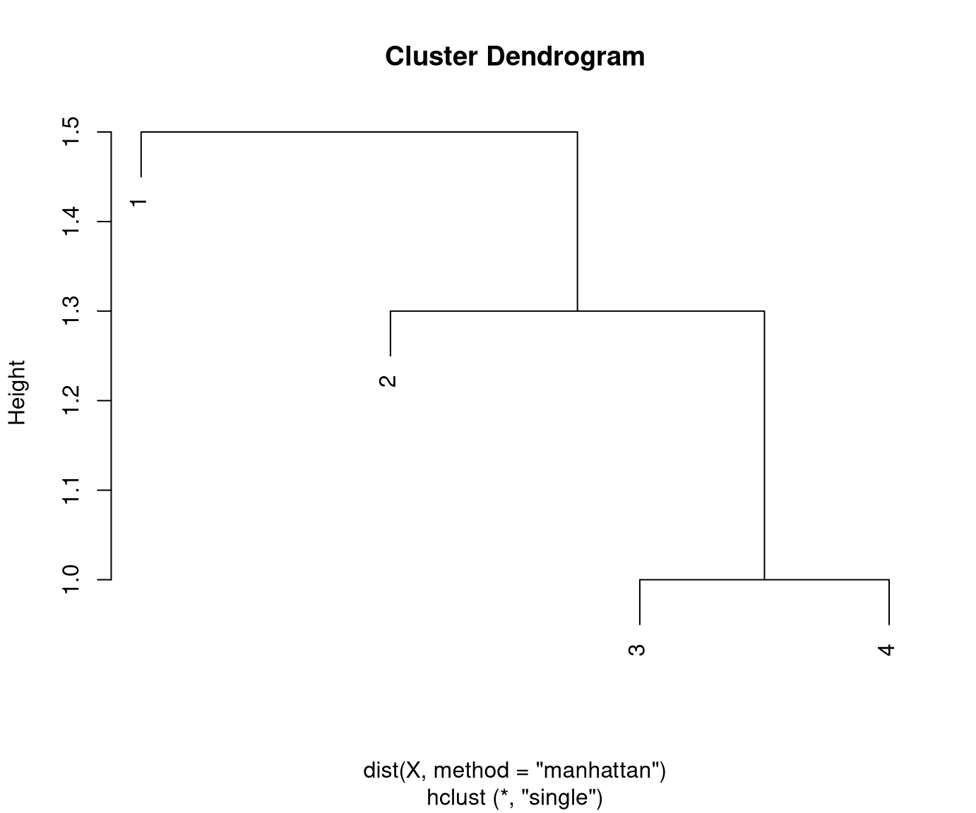
Distances between clusters: Single linkage.
Initial distances between clusters/objects:
       1   2   3
    2 1.5
    3 2.8 1.3
    4 3.8 2.3 1.0
Clusters 3 and 4 have the smallest distance (1.0) and are merged first:
        1   2
    2 1.5
  3+4 2.8 1.3
Cluster/object 2 is closest to cluster 3+4 (1.3) and are merged next:
        1
2+3+4 1.5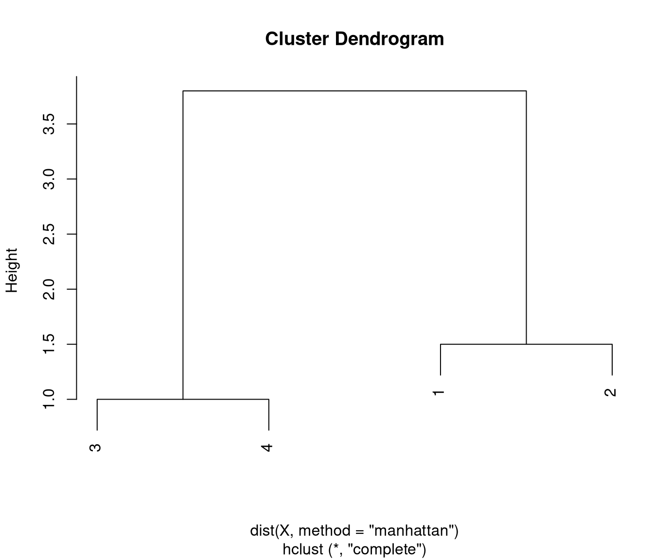
Distances between clusters: Complete linkage.
Initial distances between clusters/objects:
        1   2   3
    2 1.5
    3 2.8 1.3
    4 3.8 2.3 1.0
Clusters 3 and 4 have the smallest distance (1.0) and are merged first:
        1   2
    2 1.5
  3+4 3.8 2.3
Cluster 1 is closest to cluster 2 (1.5) and are merged next:
      1+2
  3+4 3.8


Visualization: The dendrogram displays a hierarchy of partitions by showing which clusters are merged at which distance.
Thus: The higher the step for the next merger is the more distant/dissimilar the two clusters.
Typically: Initially, the distances between merged clusters are rather low and then become larger. Stop merging when distances become “too large” to be merged.
Finally: Obtain a specific partition of the data by “cutting” the dendrogram at a certain height/distance.

Note: A partition of a data set can be employed as a new “qualitative” (or “categorical”) variable because it has partitioned the data into non-overlapping groups.
Therefore: The partition from a cluster analysis can be used for exploratory analysis of the data.
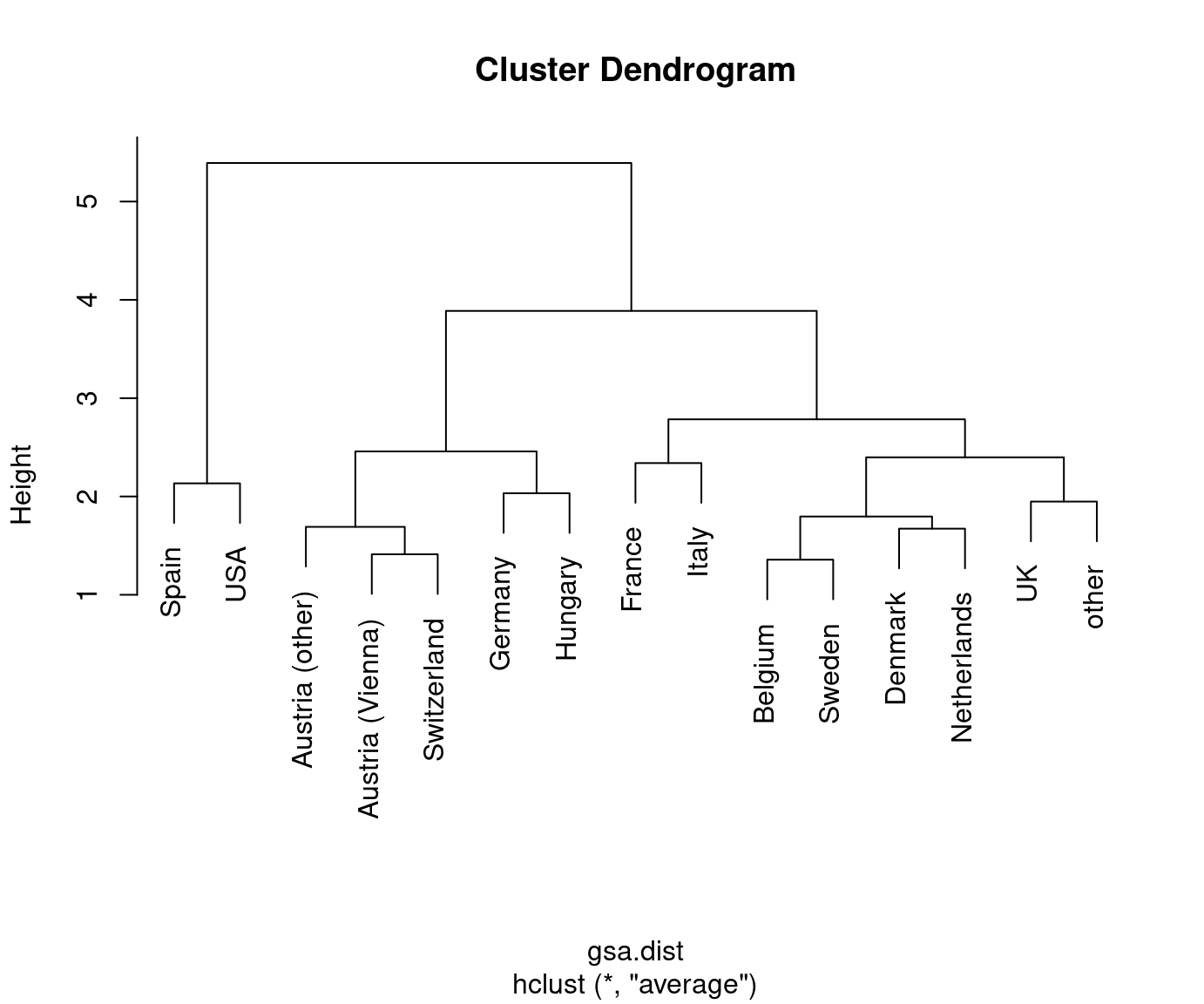
Here: Split the GSA data into three groups. Note that this was already used in a few exploratory displays above.
- Austria (Vienna), Austria (other), Germany, Hungary, Switzerland.
- Belgium, Denmark, France, Italy, Netherlands, Sweden, UK, other.
- Spain, USA.
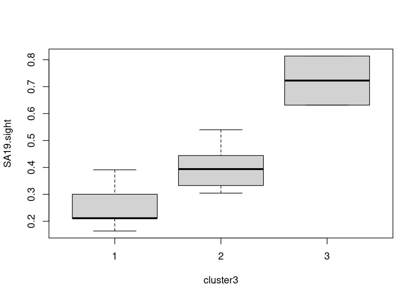
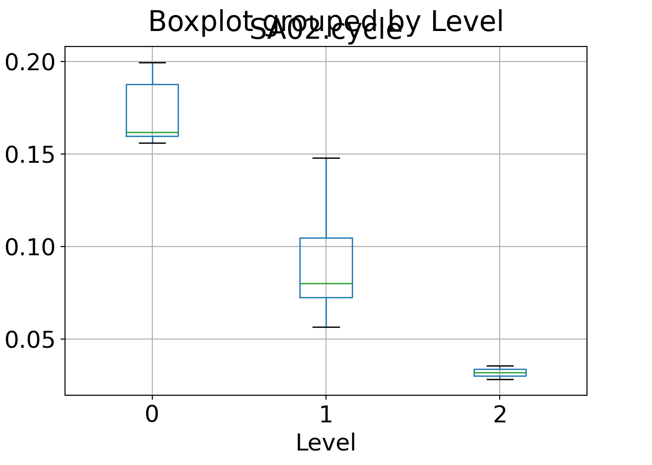
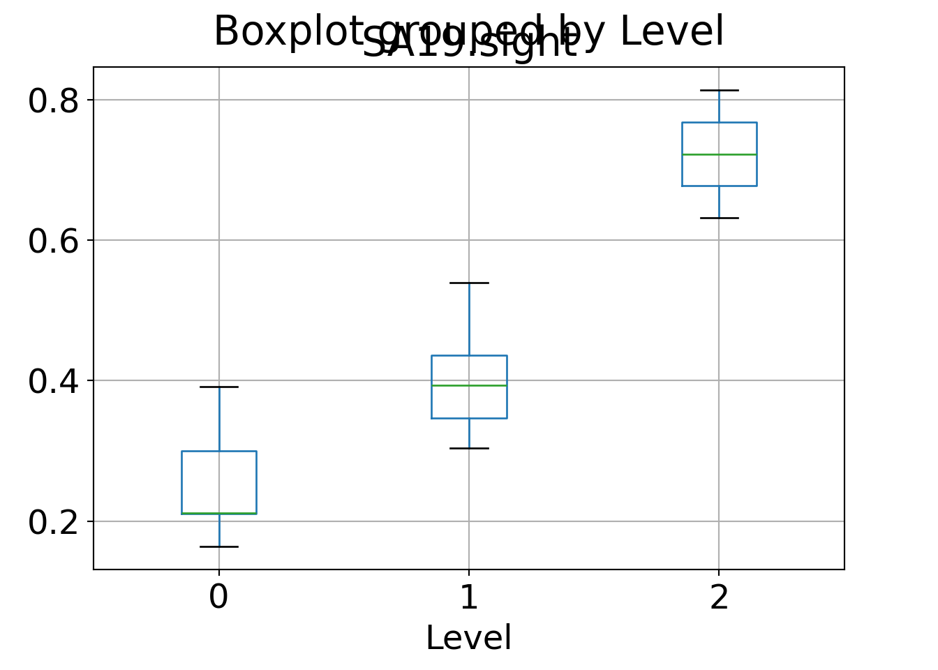
Illustration: Groupwise means and parallel boxplots.
Cycling:
##         1         2         3
## 0.1728554 0.0910864 0.0320983
Sightseeing:
##        1        2        3
## 0.255377 0.398215 0.722620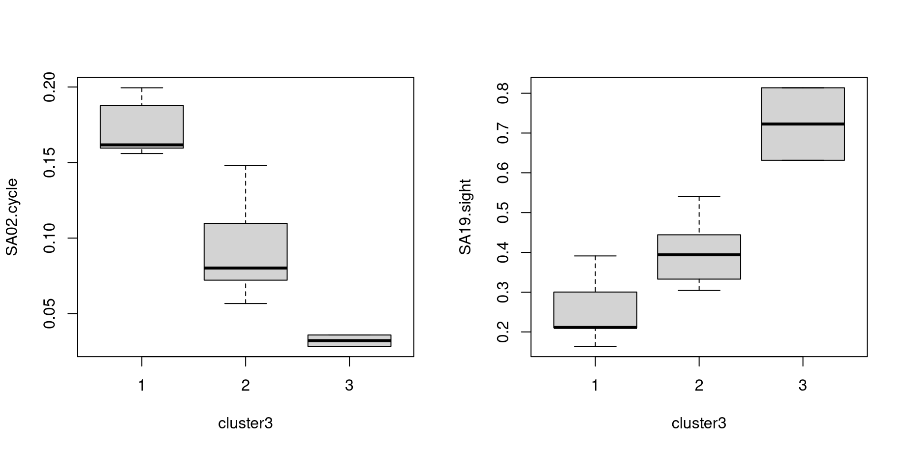
7.5 Tutorial
As in previous chapters, the Guest Survey Austria data are used for illustration, considering the interest in \(p = 8\) summer activities aggregated within \(n = 15\) countries. See Chapter 3 for the data preprocessing, or download the data set directly: gsa-country.csv, gsa-country.rda.
7.5.1 Setup
Python
# Make sure that the required libraries are installed.
# Import the necessary libraries and classes:
import pandas as pd
import numpy as np
from matplotlib import pyplot as plt
import seaborn as sns
from pca import pca

from scipy.cluster.hierarchy import dendrogram, linkage, cut_tree
from scipy.spatial.distance import pdist, squareform

pd.set_option("display.precision", 4) # Set display precision to 4 digits in pandas and numpy.
Load the gsa-country.csv dataset. See Chapter 3
for the data preprocessing and the explanations for handling the
index column.
##                   SA01.tennis  SA02.cycle  ...  SA19.sight  SA21.museum
## Country                                    ...
## Austria (Vienna)       0.0380      0.1876  ...      0.1638       0.0575
## Austria (other)        0.0399      0.1995  ...      0.2112       0.0680
## Belgium                0.0134      0.1000  ...      0.3045       0.0866
## Denmark                0.0192      0.0806  ...      0.3608       0.0787
## France                 0.0190      0.0711  ...      0.4218       0.1754
##
## [5 rows x 8 columns]
7.5.2 Clustering
Cluster the Guest Survey Austria data (Further details about distances are provided below in Chapter 7.5.4.)
R
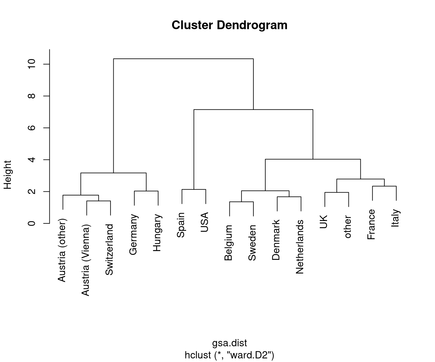
Hierarchical clustering can be easily carried out in base R using the hclust()
function based on some dissimilarity matrix, e.g., as produced by the dist()
function. Additionally, the method can be specified including: "complete"
(default), "single", and "average". For Ward’s original criterion
"ward.D2" can be specified or "ward.D" for a version based on the absolute
rather than squared dissimilarities.
Thus, we first compute the Euclidean distances of the scaled data.
Based on this we obtain a hierarchical clustering solution using average linkage:
R
##
## Call:
## hclust(d = gsa.dist, method = "average")
##
## Cluster method   : average
## Distance         : euclidean
## Number of objects: 15
The print() method only reports which configuration of arguments was
used but not what the outcome is.
Python
## [[ 2. 10. 1.35710716 2. ]
## [ 0. 11. 1.41192634 2. ]
## [ 3. 8. 1.67274596 2. ]
## [ 1. 16. 1.69109404 3. ]
## [15. 17. 1.79592175 4. ]
## [12. 14. 1.94757834 2. ]
## [ 5. 6. 2.03289573 2. ]
## [ 9. 13. 2.13373743 2. ]
## [ 4. 7. 2.33953719 2. ]
## [19. 20. 2.39845943 6. ]
## [18. 21. 2.45843347 5. ]
## [23. 24. 2.78477712 8. ]
## [25. 26. 3.88783742 13. ]
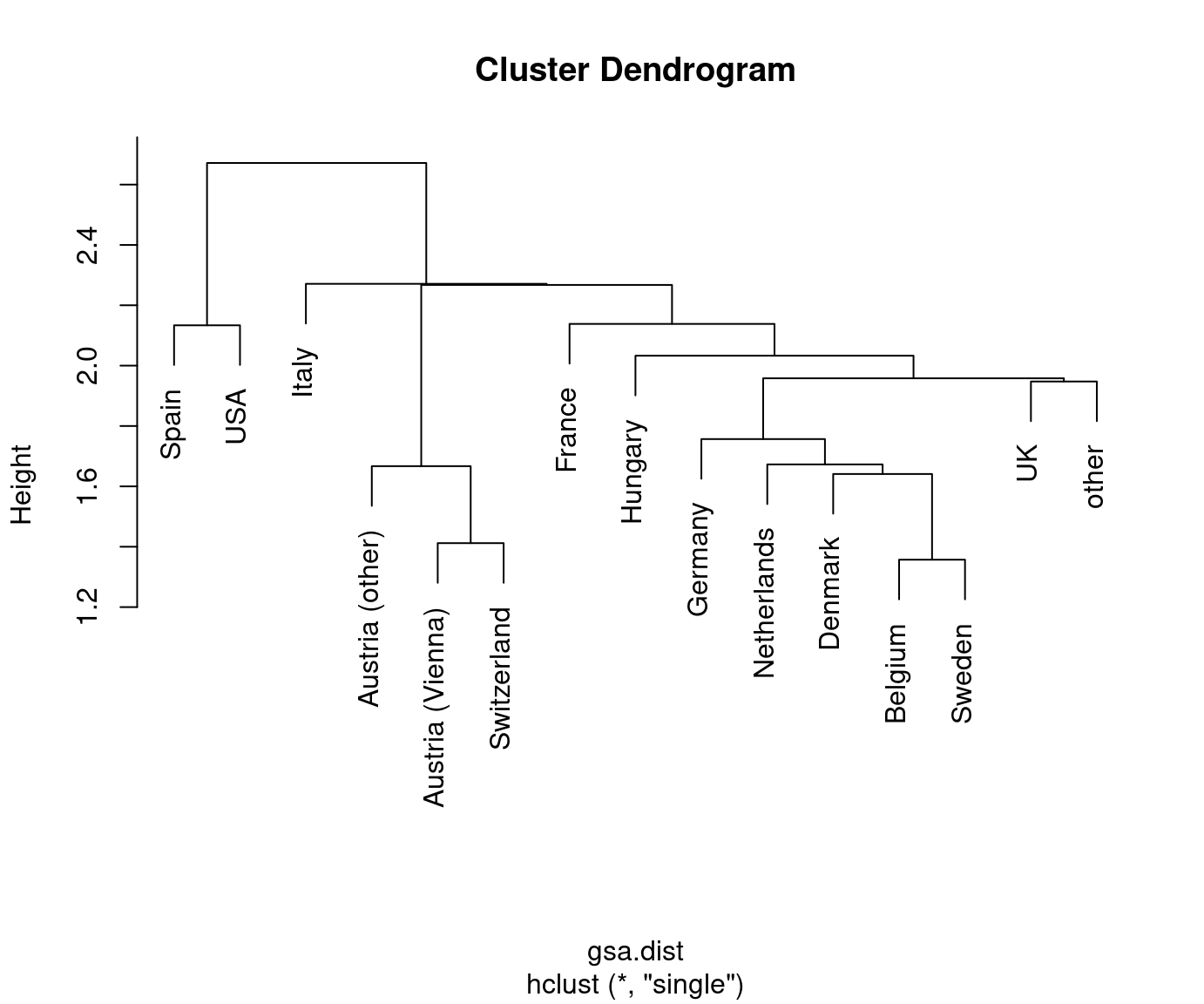
## [22. 27. 5.3920923 15. ]]Graphical overview of the results as a dendogram:


Reading this dendrogram bottom-up shows that many similar clusters are merged at
rather low heights/dissimilarities. At a height of 2.5-3.5 the additional gap
that has to be bridged for merging the next clusters becomes much larger. Thus,
it is natural to split at this height/dissimilarity into three clusters. In R, the
function rect.hclust() does so using a horizontal cut, highlighting the
resulting clusters.
In this case, the cluster with Spain and the USA is most different from the remaining two clusters Austria/Switzerland/Germany/Hungary and the remaining countries.
This also corresponds to the three clusters that are visible along the first principal component in Chapter 6 Principal component analysis. See also below for visualizations of the color-coded principal components for this data.
Possibly, we could also consider a cut into four rather than three clusters. This would additionally separate France/Italy from the remaining countries. However, these are clearly more similar (or less dissimilar) than the other two clusters.
7.5.3 Interpreting the clusters
Clustering methods yield an exhaustive and mutually exclusive split of the observations/objects into groups/clusters. Therefore, the outcome can be treated like a qualitatative or categorical variable.
R
In R the cutree() function yields an integer vector for a given number of
clusters, that can then be converted into a factor().
## Austria (Vienna)  Austria (other)          Belgium          Denmark           France
##                1                1                2                2                2
##          Germany          Hungary            Italy      Netherlands            Spain
##                1                1                2                2                3
##           Sweden      Switzerland               UK              USA            other
##                2                1                2                3                2
## Levels: 1 2 3
Python
cluster3 = pd.DataFrame({'Country': country_labels, 'Level': cut_tree(hclust, height=3)[:, 0]})

print(cluster3)
## Country Level
## 0 Austria (Vienna) 0
## 1 Austria (other) 0
## 2 Belgium 1
## 3 Denmark 1
## 4 France 1
## 5 Germany 0
## 6 Hungary 0
## 7 Italy 1
## 8 Netherlands 1
## 9 Spain 2
## 10 Sweden 1
## 11 Switzerland 0
## 12 UK 1
## 13 USA 2
## 14 other 1Subsequent analysis can then employ the same ideas as discussed in Chapter 4 based on qualitative variables. For example, we can compute group-wise statistics or parallel boxplots etc. to characterize how the interest in the summer activities differs across clusters.
For example, we can summarize the mean interest in a particular summer activity (here: cycling) across clusters:
This shows very high interest in cluster 1 (R) / cluster 0 (Python) (Austria/…), moderate interest in cluster 2 (R) / cluster 1 (Python) (other), and low interest in cluster 3 (R) / cluster 2 (Python) (Spain/USA). We can do the same for all variables simultaneously, either for the raw original data or the scaled data (with zero mean and unit variance):
R
##   Group.1 SA01.tennis SA02.cycle   SA03.ride SA05.swim SA17.shop SA18.concert SA19.sight
## 1       1  0.03281770  0.1728554 0.010811730  0.396356  0.122779    0.0232550   0.255377
## 2       2  0.01724108  0.0910864 0.002581565  0.307048  0.206973    0.0461825   0.398215
## 3       3  0.00501234  0.0320983 0.000996016  0.118336  0.252803    0.0822540   0.722620
##   SA21.museum
## 1   0.0840328
## 2   0.1317405
## 3 0.3378873## Group.1 SA01.tennis SA02.cycle SA03.ride SA05.swim SA17.shop SA18.concert SA19.sight
## 1 1 0.993413 1.131318 1.153165 0.8135672 -1.091354 -0.832119 -0.8122326
## 2 2 -0.294488 -0.351691 -0.512408 -0.0442605 0.384957 0.117313 0.0255657
## 3 3 -1.305580 -1.421533 -0.833282 -1.8568762 1.188556 1.611043 1.9283186
## SA21.museum
## 1 -0.569453
## 2 -0.111253
## 3 1.868646Python
##        SA01.tennis  SA02.cycle  ...  SA19.sight  SA21.museum
## Level                           ...
## 0           0.0328      0.1729  ...      0.2554       0.0840
## 1           0.0172      0.0911  ...      0.3982       0.1317
## 2           0.0050      0.0321  ...      0.7226       0.3379
##
## [3 rows x 8 columns]normalized_gsa.reset_index(inplace=True)
normalized_gsa["Level"] = cluster3["Level"]
normalized_gsa.set_index("Country", inplace=True)
print(normalized_gsa.groupby(["Level"]).mean())## SA01.tennis SA02.cycle ... SA19.sight SA21.museum
## Level ...
## 0 0.9934 1.1313 ... -0.8122 -0.5695
## 1 -0.2945 -0.3517 ... 0.0256 -0.1113
## 2 -1.3056 -1.4215 ... 1.9283 1.8686
##
## [3 rows x 8 columns]The latter is also straightforward to interpret here: Cluster 1 (0 in Python) has rather high interest (around one standard deviation above average) in the sports activities but rather low interest (close to one standard deviation below average) in the cultural activities. In cluster 3 (2 in Python) this pattern is reversed and even more pronounced (up to two standard deviations). Cluster 2 (1 in Python) is in between with roundabout average interest (i.e., zero on the standardized scale) for all activities.
Graphically, box plots could be used to bring out the same:

Finally, as mentioned already above, we can also highlight that the groups found by hierarchical clustering match what we have concluded from the Principal component analysis (PCA) for these data. To do so, we re-generated the PCA, predict the first two principal components, and color-code the clusters in the corresponding scatter plot:
R
gsa.pc <- prcomp(gsa, scale = TRUE)
gsa.pc <- predict(gsa.pc)[, 1:2]
gsa.cl <- hcl.colors(3, "Dark 3")[cluster3]
plot(gsa.pc[, 1:2], type = "n", xlab = "PC1", ylab = "PC2",
  xlim = c(-4.5, 4.5), ylim = c(-4.5, 4.5))
text(gsa.pc[, 1:2], rownames(gsa), col = gsa.cl)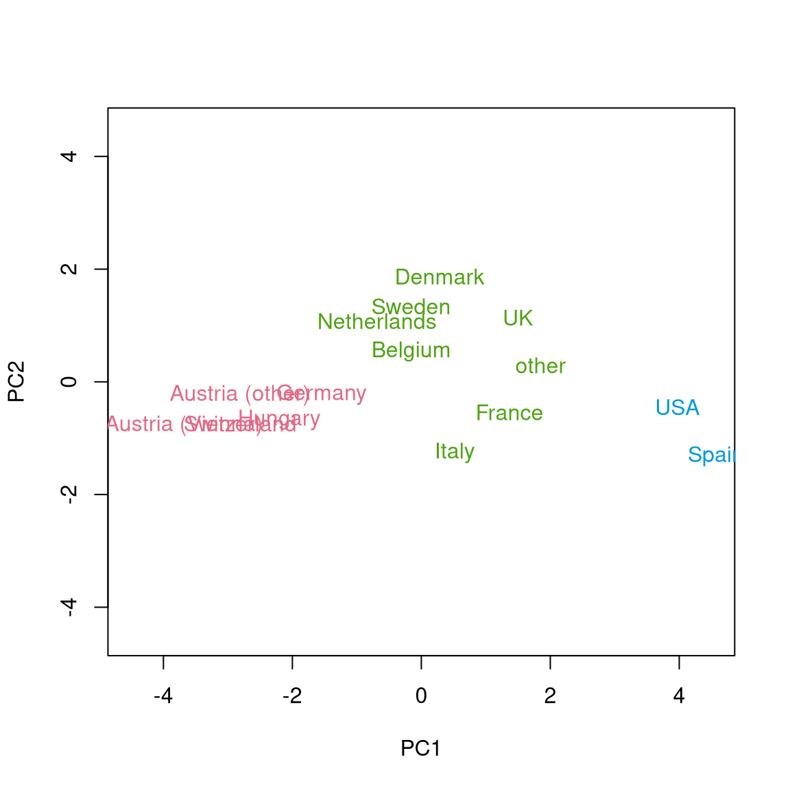
The corresponding
three colors are generated by hcl.colors() from the "Dark 3" palette and
then assigned to the clusters by indexing with the factor cluster3.
Python
gsa.drop(["Level"], axis=1, inplace=True)
normalized_gsa = (gsa-gsa.mean())/gsa.std()

gsa_pca = pca(n_components=8, normalize=False)
pca_results = gsa_pca.fit_transform(normalized_gsa, verbose=0)
pc = gsa_pca.results['PC'].iloc[:, 0:2]

fig = plt.figure()
ax = plt.axis([-5.5, 5.5, -5.5, 5.5])
colors = plt.cm.get_cmap("rainbow", 3)
## <string>:1: MatplotlibDeprecationWarning: The get_cmap function was deprecated in Matplotlib 3.7 and will be removed in 3.11. Use ``matplotlib.colormaps[name]`` or ``matplotlib.colormaps.get_cmap()`` or ``pyplot.get_cmap()`` instead.cluster3.set_index("Country", inplace=True)
for index, row in pc.iterrows():
color = colors(cluster3.loc[index][0])
plt.text(row["PC1"], row["PC2"], index, {"color": color})
plt.xlabel("PC1")
plt.ylabel("PC2")
plt.show()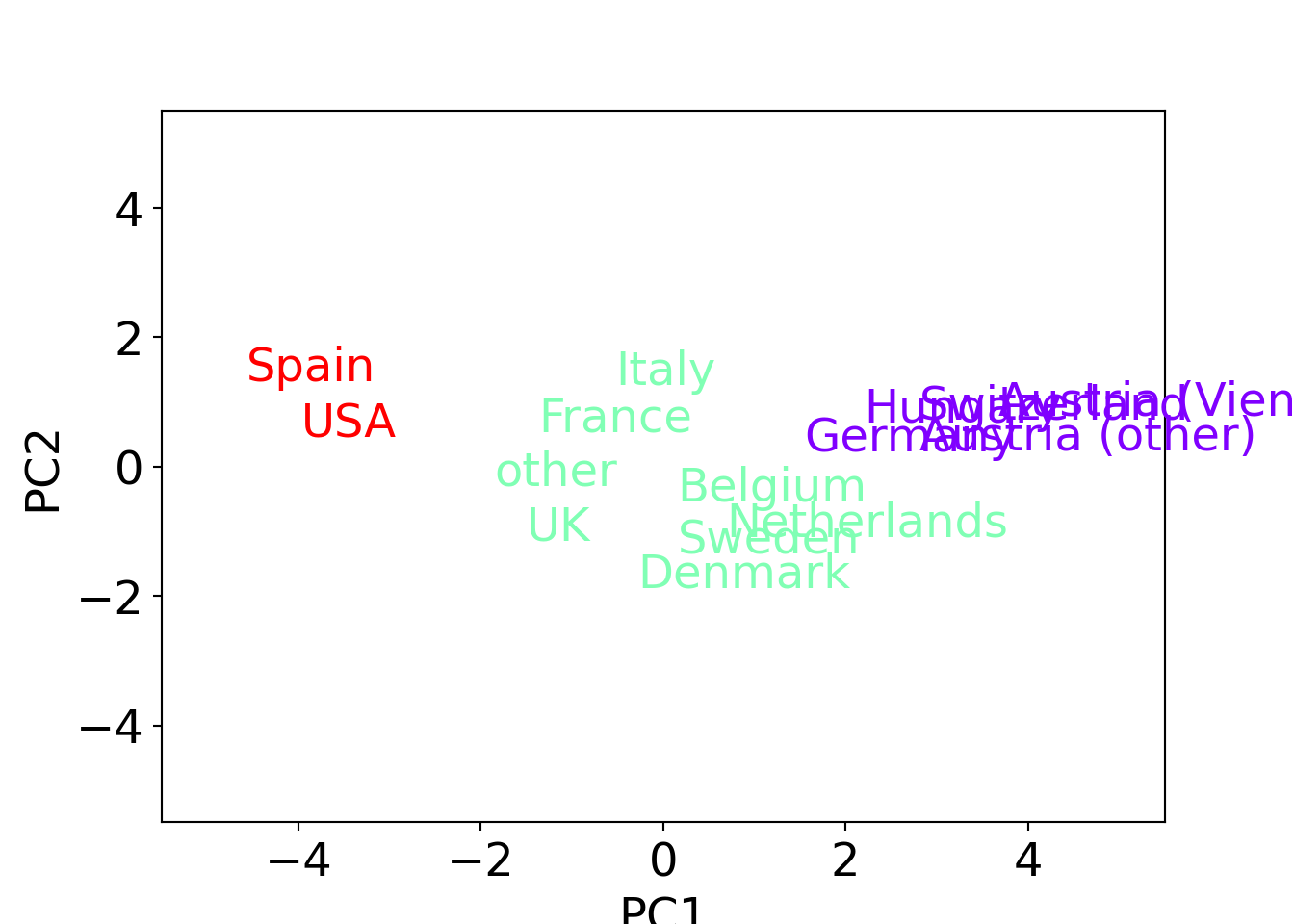
This shows that the differences along the first principal component (sports vs. cultural interests) drive the split into the three clusters.
7.5.4 Distances
To illustrate how the function works we consider only the first five countries from the scaled Guest Survey Austria data.
R
Hierarchical clustering with hclust() in R is based on a dissimilarity
specification, e.g., as produced by the dist() function. The latter can take
an \(n \times p\) data matrix and computes the lower triangular matrix of the
corresponding \(n \times n\) distance matrix. The most common distance methods
for quantitative data are supported: "euclidean", "manhattan", "maximum",
and "canberra". Furthermore, the standard "binary" distance is also
available.
##                  SA01.tennis SA02.cycle SA03.ride  SA05.swim  SA17.shop SA18.concert
## Austria (Vienna)    1.418665   1.399380  1.599087  0.9860827 -1.7418195   -1.1214115
## Austria (other)     1.578261   1.613763  0.066007  0.7510348 -1.2570920   -0.7439020
## Belgium            -0.609360  -0.190029  0.173354  0.0600785 -0.0251994    0.0590759
## Denmark            -0.133029  -0.541621 -1.034850  0.6015232  1.2656237   -0.6823627
## France             -0.152584  -0.714357 -0.715143 -0.5808363 -0.5018608    1.7375131
##                  SA19.sight SA21.museum
## Austria (Vienna)  -1.349519   -0.824439
## Austria (other)   -1.071103   -0.723472
## Belgium           -0.524242   -0.545113
## Denmark           -0.193629   -0.620721
## France             0.163904    0.307638
Python
##                   SA01.tennis  SA02.cycle  ...  SA19.sight  SA21.museum
## Country                                    ...
## Austria (Vienna)       1.4187      1.3994  ...     -1.3495      -0.8244
## Austria (other)        1.5783      1.6138  ...     -1.0711      -0.7235
## Belgium               -0.6094     -0.1900  ...     -0.5242      -0.5451
## Denmark               -0.1330     -0.5416  ...     -0.1936      -0.6207
## France                -0.1526     -0.7144  ...      0.1639       0.3076
##
## [5 rows x 8 columns]
Using different method (in R) or metric (in Python) specifications we get:
R
##                 Austria (Vienna) Austria (other) Belgium Denmark
## Austria (other)          1.71528
## Belgium                  3.82475         3.31986
## Denmark                  4.88629         3.99460 2.10580
## France 5.29439 4.48512 2.43492 3.39115## Austria (Vienna) Austria (other) Belgium Denmark
## Austria (other) 3.38373
## Belgium 9.97088 7.54981
## Denmark 11.31729 8.68152 5.01605
## France 14.31052 11.67475 6.20651 7.16761These are represented as lower triangular matrices because the main diagonal is
by definition 0 and the matrix is symmetric. If needed, a full matrix can be
easily set up with as.matrix():
##                  Austria (Vienna) Austria (other) Belgium Denmark  France
## Austria (Vienna)          0.00000         1.71528 3.82475 4.88629 5.29439
## Austria (other)           1.71528         0.00000 3.31986 3.99460 4.48512
## Belgium                   3.82475         3.31986 0.00000 2.10580 2.43492
## Denmark                   4.88629         3.99460 2.10580 0.00000 3.39115
## France                    5.29439         4.48512 2.43492 3.39115 0.00000
Such a full distance matrix (either from dist() or computed by some other
means) can also be passed to hclust() as the main argument.
Python
Show the distance vector computed by pdist().
## [1.71528328 3.82475447 4.88628823 5.29439342 3.31986442 3.99460095
##  4.48511667 2.10580248 2.43492269 3.39114835]
Make a nicer visualization
labels, indices = np.unique(sgsa5.index, return_inverse=True)
country_labels = labels[indices]

dist_matrix = pd.DataFrame(squareform(D), index=country_labels, columns=country_labels)
print(dist_matrix)
## Austria (Vienna) Austria (other) Belgium Denmark France
## Austria (Vienna) 0.0000 1.7153 3.8248 4.8863 5.2944
## Austria (other) 1.7153 0.0000 3.3199 3.9946 4.4851
## Belgium 3.8248 3.3199 0.0000 2.1058 2.4349
## Denmark 4.8863 3.9946 2.1058 0.0000 3.3911
## France 5.2944 4.4851 2.4349 3.3911 0.0000D = pdist(sgsa5, metric='cityblock')
dist_matrix = pd.DataFrame(squareform(D), index=country_labels, columns=country_labels)
print(dist_matrix)## Austria (Vienna) Austria (other) Belgium Denmark France
## Austria (Vienna) 0.0000 3.3837 9.9709 11.3173 14.3105
## Austria (other) 3.3837 0.0000 7.5498 8.6815 11.6748
## Belgium 9.9709 7.5498 0.0000 5.0161 6.2065
## Denmark 11.3173 8.6815 5.0161 0.0000 7.1676
## France 14.3105 11.6748 6.2065 7.1676 0.0000