Chapter 18 Generalized linear models
18.1 Model frame
Model equation: The generalized linear model (GLM) is given by
\[\begin{eqnarray*} \text{E}(y_i) & = & \mu_i, \\ g(\mu_i) & = & x_i^\top \beta, \end{eqnarray*}\]
where
- \(y_i\): Random variable from an exponential family (e.g., normal/Gaussian, binomial, Poisson) with expectation \(\mu_i\).
- \(g(\cdot)\): Link function mapping the scale of the expectation \(\mu_i\) to the scale of the linear predictor (real line).
- \(x_i\): Regressor vector of explanatory variables.
- \(\beta\): Vector of corresponding coefficients.
Formally: A random variable \(y\) follow an exponential family if the probability density function is of the following type:
\[ f(y ~|~ \theta, \phi) ~=~ \exp\left(\frac{y \cdot \theta - a(\theta)}{\phi} ~+~ b(y, \phi) \right) \]
where \(a(\cdot)\) and \(b(\cdot)\) are known functions, \(\phi\) is a (potentially known) dispersion parameter and \(\theta\) is the so-called canonical parameter.
Special cases:
- Normal or Gaussian distribution.
- Binomial distribution.
- Poisson distribution.
Estimation: After fixing the concrete distribution of \(y_i\) the complete likelihood \(\ell(\beta)\) is specified up to the unknown coefficients \(\beta\) which can thus be estimated by maximum likelihood (ML).
Algorithm: As the MLE typically cannot be computed in closed form (except in special cases), an iterative numeric algorithm is used. This is known as iteratively weighted least squares (IWLS).
Objective function: Log-likelihood. In the statistics literature the so-called deviance is used equivalently which is typically essentially \(-2 \cdot \ell(\hat \beta)\). The deviance has properties similar to the residual sum of squares in the linear regression model.
Prediction: Expected values \(\hat \mu_i\) can be computed by applying the inverse link function to the linear predictor with estimated coefficients
\[ \hat \mu_i ~=~ g^{-1} \left( x_i^\top \hat \beta \right). \]
Residuals: In the linear regression model it was reasonable to simply employ the prediction errors \[ y_i - \hat \mu_i \]
as it was assumed that the corresponding variances are (approximately) constant.
Scaling: The GLM is often (by construction) heteroscedastic and hence residuals should be scaled suitably, e.g., by their standard deviation.
Pearson residuals:
\[ \frac{y_i - \hat \mu_i}{\sqrt{\text{Var}(\hat \mu_i)}} \]
The variance function is proportional to the variance of \(y_i\) and given by:
- Normal: \(\text{Var}(\mu) = 1\).
- Binomial: \(\text{Var}(\mu) = \mu \cdot (1 - \mu)\).
- Poisson: \(\text{Var}(\mu) = \mu\).
Alternatively: Other useful definitions of residuals in GLMs exist, e.g., deviance residuals which are computed by default in R.
18.2 Special cases
Linear regression: Is a special case of GLMs when assuming that \(y_i\) is normally independently distributed with equal variance.
Canonical link function: Identity \(g(\mu) = \mu\).
Remark: This corresponds exactly to assumptions (A1)–(A6).
Poisson regression: The basic distribution for modeling count data is the Poisson distribution.
Canonical link function: Logarithm \(g(\mu) = \log(\mu)\).
Binomial regression: For binary dependent variables the Bernoulli distribution is used, which is the special case of the binomial distribution.
Canonical link function: Logit function corresponding to modeling log-odds \[ g(\mu) ~=~ \log \left( \frac{\mu}{1-\mu} \right). \]
Alternatively: Probit link function \[ g(\mu) ~=~ \Phi^{-1} (\mu) \] where \(\Phi(\cdot)\) is the standard normal cumulative distribution function.
Motivation:
- Model discrete choice of a customer for testing a certain product.
- It is assumed that the customer only tests the product if advertising exceeds a certain individual threshold.
- Thresholds vary across customers following a normal distribution with expectation \(m\) and variance \(s^2\): \(T \sim \mathcal{N}(m, s^2)\).
Choice probability: Follows binary GLM with probit link.
\[\begin{eqnarray*} \mu ~=~ \text{P}(T \le \mathsf{Advertising}) & = & \Phi \left( \frac{\mathsf{Advertising} - m}{s} \right) \\ \Phi^{-1} \left( \mu \right) & = & -\frac{m}{s} + \frac{1}{s} \cdot \mathsf{Advertising} \\ & = &\beta_1 + \beta_2 \cdot \mathsf{Advertising} \end{eqnarray*}\]
18.3 Related methods
Discrete choice models:
- Multinomial model: Similar to binomial model but the dependent variable can have \(c > 2\) levels.
- Ordered logistic regression: Or proportional odds model. The dependent variable has \(c > 2\) ordered levels (e.g., ratings).
- Conjoint analysis: Similar to multinomial model but each choice is made only between less than all \(c\) levels.
Count data regression: In many fields like economics or social sciences count data have dispersion higher than in the Poisson model with many more zeros.
- Negative binomial model.
- Zero-inflated model.
- Hurdle model.
Prediction vs. probabilistic explanation: If only prediction is the focus, then predictive algorithmic models from machine learning and statistical learning often perform very well.
- Tree-based: Classification and regression trees, bagging, random forests.
- Gradient boosting.
- Neural networks and deep learning.
- Support vector machines.
18.4 Tutorial
For illustrating generalized linear models (GLMs) with non-Gaussian dependent
variables the Bookbinder’s Book Club case study is employed. The BBBClub data set can be downloaded as BBBClub.csv or BBBClub.rda. For an exploratory
data analysis of the data see Chapter 4. In this chapter, although the case study was not designed for this task, the data is used to model a count response
(the number of purchased child books) using Poisson regression.
18.4.1 Setup
Python
# Make sure that the required libraries are installed.
# Import libraries and classes:
import pandas as pd
import numpy as np
import matplotlib.pyplot as plt
import seaborn as sns
import statsmodels.api as sm
import statsmodels.formula.api as smf
from itertools import combinations
from statsmodels.graphics.mosaicplot import mosaic

from stepwise_selection import stepwise_selection, update_model

pd.set_option("display.precision", 4) # Set display precision to 4 digits in pandas and numpy.18.4.2 Poisson regression
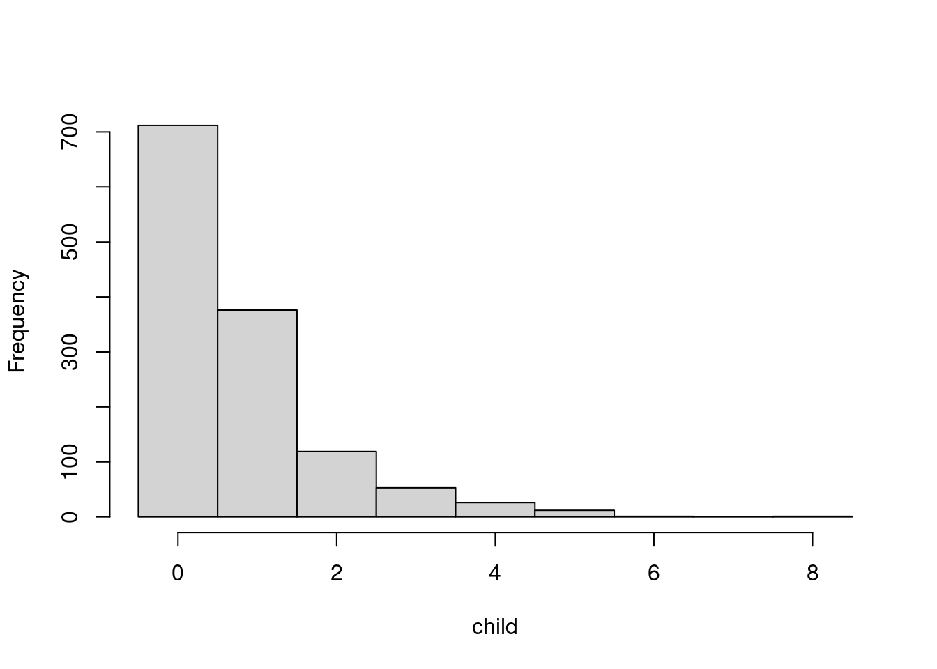
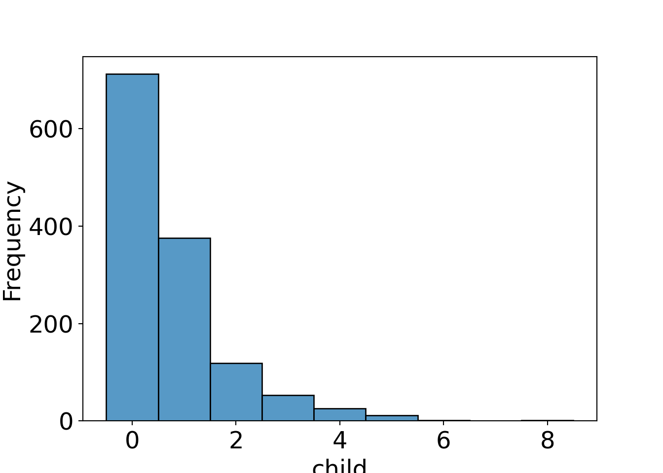
Question: Which variables in the Bookbinder’s Book Club data determine the number of children’s books bought by the customers?
Histogram: Number of children’s books purchased
Plot: Number of purchased child books ~ amount and last purchase
R
plot(jitter(child) ~ amount, data = BBBClub, ylim = c(-0.5, 8.5))
plot(jitter(child) ~ jitter(last), data = BBBClub, ylim = c(-0.5, 8.5), xlim = c(0.5, 12.5))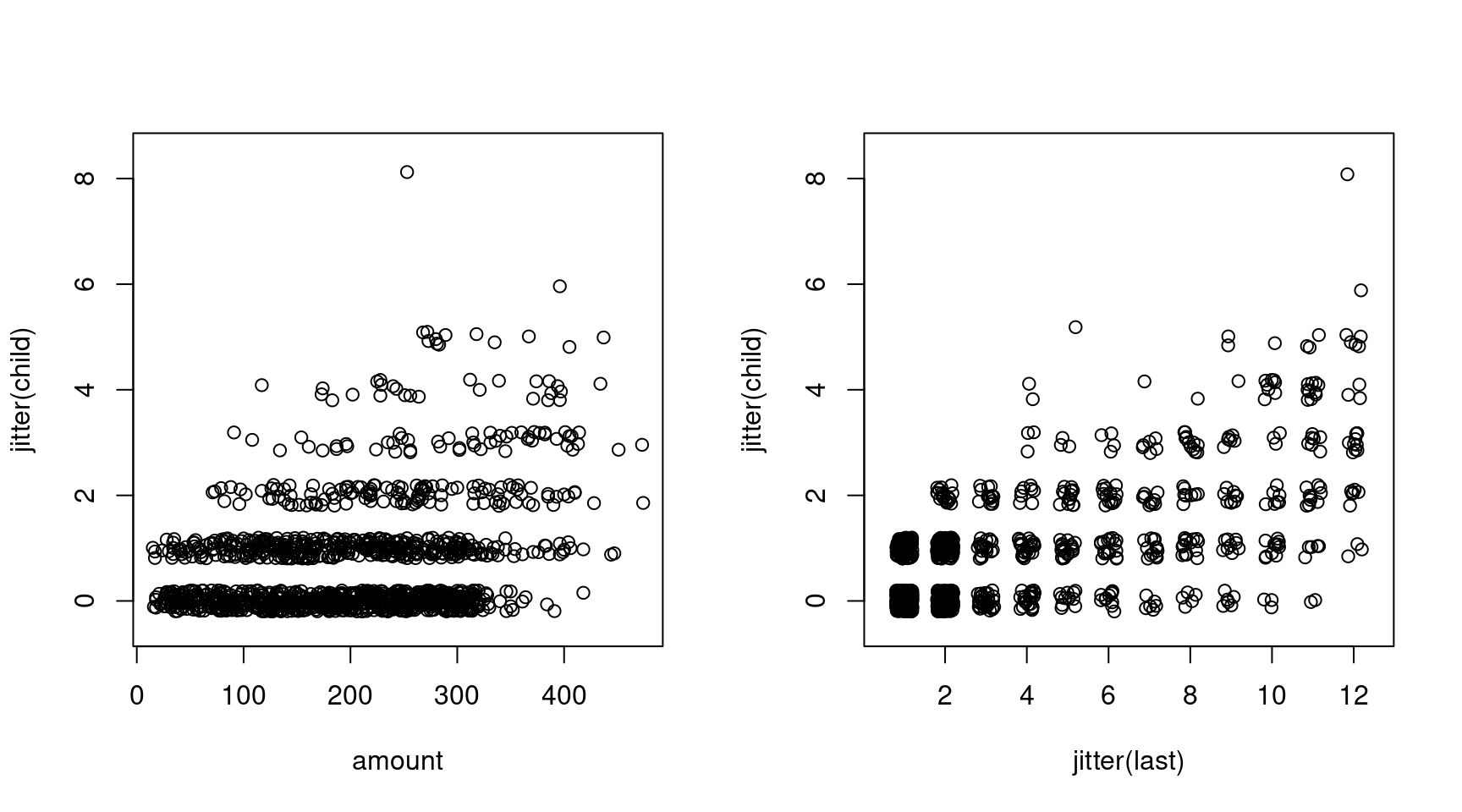


Illustration: Backward selection starting from gender interaction model.
R
m1 <- glm(child ~ gender * (amount + first + last + freq),
  data = BBBClub, family = poisson)
m2 <- step(m1)
## Start: AIC=2498
## child ~ gender * (amount + first + last + freq)
##
## Df Deviance AIC
## - gender:first 1 1122 2496
## - gender:freq 1 1123 2496
## - gender:last 1 1123 2497
## <none> 1122 2498
## - gender:amount 1 1127 2501
##
## Step: AIC=2496
## child ~ gender + amount + first + last + freq + gender:amount +
## gender:last + gender:freq
##
## Df Deviance AIC
## - gender:freq 1 1123 2494
## - first 1 1123 2495
## <none> 1122 2496
## - gender:last 1 1126 2498
## - gender:amount 1 1127 2499
##
## Step: AIC=2494
## child ~ gender + amount + first + last + freq + gender:amount +
## gender:last
##
## Df Deviance AIC
## - first 1 1123 2493
## - freq 1 1123 2493
## <none> 1123 2494
## - gender:last 1 1126 2496
## - gender:amount 1 1127 2497
##
## Step: AIC=2493
## child ~ gender + amount + last + freq + gender:amount + gender:last
##
## Df Deviance AIC
## - freq 1 1123 2491
## <none> 1123 2493
## - gender:last 1 1127 2494
## - gender:amount 1 1127 2495
##
## Step: AIC=2491
## child ~ gender + amount + last + gender:amount + gender:last
##
## Df Deviance AIC
## <none> 1123 2491
## - gender:last 1 1127 2493
## - gender:amount 1 1128 2494Python
Poisson regression
formula = "child ~ gender * (amount + first + last + freq)"

m1 = smf.glm(formula=formula, data=BBBClub, family=sm.families.Poisson())

m2 = stepwise_selection(m1)
## Step: aic= 2498.3113199595036
## (' - gender:first', np.float64(2496.349604965202))
## (' - gender:freq', np.float64(2496.4864095144194))
## (' - gender:last', np.float64(2496.9984234172807))
## ('', np.float64(2498.3113199595036))
## (' - gender:amount', np.float64(2500.7849047936834))
## Step: aic= 2496.349604965202
## (' - gender:freq', np.float64(2494.4941663409636))
## (' - first', np.float64(2494.6577861257106))
## ('', np.float64(2496.349604965202))
## (' - gender:last', np.float64(2497.6517997369765))
## (' + gender:first', np.float64(2498.3113199595036))
## (' - gender:amount', np.float64(2498.809845986335))
## Step: aic= 2494.4941663409636
## (' - first', np.float64(2492.780949479548))
## (' - freq', np.float64(2493.278927417289))
## ('', np.float64(2494.4941663409636))
## (' - gender:last', np.float64(2495.99240630355))
## (' + gender:freq', np.float64(2496.349604965202))
## (' + gender:first', np.float64(2496.4864095144194))
## (' - gender:amount', np.float64(2497.069228926175))
## Step: aic= 2492.780949479548
## (' - freq', np.float64(2491.28009017402))
## ('', np.float64(2492.780949479548))
## (' - gender:last', np.float64(2494.4936804179106))
## (' + first', np.float64(2494.4941663409636))
## (' + gender:freq', np.float64(2494.6577861257106))
## (' - gender:amount', np.float64(2495.3531813595264))
## (' + gender:first', np.float64(2496.48640951442))
## Step: aic= 2491.28009017402
## ('', np.float64(2491.28009017402))
## (' + freq', np.float64(2492.780949479548))
## (' - gender:last', np.float64(2493.015294624491))
## (' + first', np.float64(2493.2789274172887))
## (' - gender:amount', np.float64(2493.869335358124))
## (' + gender:freq', np.float64(2494.657786125711))
## (' + gender:first', np.float64(2495.2770397931135))
## Result: aic= 2491.28009017402
## child ~ gender + amount + last + gender:amount + gender:lastSummary of the model selected by stepwise selection:
R
##
## Call:
## glm(formula = child ~ gender + amount + last + gender:amount +
##     gender:last, family = poisson, data = BBBClub)
##
## Coefficients:
##                    Estimate Std. Error z value Pr(>|z|)
## (Intercept)       -1.401280   0.141544   -9.90   <2e-16
## gendermale         0.088767   0.176459    0.50    0.615
## amount             0.001307   0.000620    2.11    0.035
## last               0.189938   0.016125   11.78   <2e-16
## gendermale:amount -0.001684   0.000788   -2.14    0.033
## gendermale:last    0.038691   0.020066    1.93    0.054
##
## (Dispersion parameter for poisson family taken to be 1)
##
##     Null deviance: 1810.1  on 1299  degrees of freedom
## Residual deviance: 1123.4  on 1294  degrees of freedom
## AIC: 2491
##
## Number of Fisher Scoring iterations: 5
Python
##                  Generalized Linear Model Regression Results
## ==============================================================================
## Dep. Variable:                  child   No. Observations:                 1300
## Model:                            GLM   Df Residuals:                     1294
## Model Family:                 Poisson   Df Model:                            5
## Link Function:                    Log   Scale:                          1.0000
## Method:                          IRLS   Log-Likelihood:                -1239.6
## Date:                Wed, 05 Mar 2025   Deviance:                       1123.4
## Time:                        14:24:03   Pearson chi2:                 1.05e+03
## No. Iterations:                     5   Pseudo R-squ. (CS):             0.4104
## Covariance Type:            nonrobust
## =========================================================================================
##                             coef    std err          z      P>|z|      [0.025      0.975]
## -----------------------------------------------------------------------------------------
## Intercept                -1.4013      0.142     -9.900      0.000      -1.679      -1.124
## gender[T.male]            0.0888      0.176      0.503      0.615      -0.257       0.435
## amount                    0.0013      0.001      2.109      0.035    9.25e-05       0.003
## gender[T.male]:amount    -0.0017      0.001     -2.138      0.033      -0.003      -0.000
## last                      0.1899      0.016     11.779      0.000       0.158       0.222
## gender[T.male]:last       0.0387      0.020      1.928      0.054      -0.001       0.078
## =========================================================================================