Chapter 8 \(k\)-means clustering
8.1 Motivation
Idea: Instead of constructing a hierarchy of partitions, construct only one partition with a given number of \(k\) clusters directly.
Question: Which partition to choose out of all possible partitions into \(k\) clusters for \(n\) objects?
Answer: Adopt an objective function and choose that partition for which this is optimized.
Follow-up questions:
- Which objective function should be used?
- How should it be optimized? (Exhaustive search will only be feasible for small \(n\).)
Question: Which objective function should be used?
Answer: If data are quantitative, it is natural to use error sums of squares \(\mathit{SS}\). This is the sum of squared Euclidean distances of the individual observations from the corresponding cluster means.
Formally: Mean in cluster \(j\):
\[ \overline x_j \quad = \quad \frac{1}{|C_j|} \sum_{x \in C_j} x \]
Formally: Within sum of squares in cluster \(j\) and total within sum of squares.
\[\begin{eqnarray*} \mathit{WSS}(C_j) & = & \sum_{x \in C_j} d_2(x, \overline x_j)^2 \\ \mathit{SS}(\mathcal{C}) & = & \sum_{j = 1}^k \mathit{WSS}(C_j) \end{eqnarray*}\]
Jargon:
- The \(k\) means \(\overline x_1, \dots, \overline x_k\) defining partition \(\mathcal{C}\) are also known as prototypes.
- The partition \(\mathcal{C}\) (or equivalently: the corresponding \(k\) means), that minimizes the error sum of squares \(\mathit{SS}(\mathcal{C})\), is also known as \(k\)-means partition.
8.2 Algorithm
Question: In principle one go through all \(n \choose k\) possible partitions into \(k\) clusters for \(n\) objects. However, this is not feasible for large \(n\). Are there faster algorithms?
Answer: Yes, there are various algorithms for obtaining an approximative solution for the \(k\)-means problem such as the following.
- Start with \(k\) randomly-selected means \(\overline x_j\).
- Assign each observation \(x_i\) to the cluster \(j\) whose corresponding mean \(\overline x_j\) is closest.
- Compute the new means \(\overline x_j\) by taking averages in each cluster \(j\).
- Repeat steps 2 and 3 until the clusters do not change.
Problem: This algorithm is not guaranteed to find the global minimum for \(SS(\mathcal{C})\) but only a local minimum.
Example: Two different runs of \(k\)-means with different starting values for the scaled GSA data.
Remark: The following visualization of the partition uses the first two principal components. The sums of squares are computed in \(\mathbb{R}^8\) but are reflected well in the projection to \(\mathbb{R}^2\).
8.3 Interpretation
Due to different starting values different partitions are obtained. At least one of these has to be only a local minimum.
Here: The second partition \(\mathcal{C}_2\) is to be preferred because
\[\begin{eqnarray*} \mathit{SS}(\mathcal{C}_1) & = & 30.723 \mathit{SS}(\mathcal{C}_2) & = & 24.565 \end{eqnarray*}\]
In practice: Compute \(20\) (or \(50\) or \(\dots\)) partitions with different starting values and only keep the one with the smallest total within sum of squares.
Question: Which number of clusters \(k\) should be used?
Answer: Keep increasing the number of clusters \(k = 1, 2, 3, \dots\) as long as the total within sum of squares drops “clearly” for an additional cluster.
Follow-up question: What is “clearly”?
Answer: No universally accepted answer. Here, we judge this graphically based on the bar plot for the sums of squares.
Here: Choose at least \(k = 3\) clusters, maybe even \(4\).

Alternatively: There is a wide range of cluster indices that has been proposed in the literature. All of these make some form of trade-off between the number of clusters \(k\) (complexity) and homogeneity within / heterogeneity between the clusters (goodness of fit).
Then: Choose the number of clusters \(k\) that optimizes a given cluster index.
However: No universally accepted “best” cluster index. Hence not pursued in detail here.
8.4 Illustration

\(3\)-means solution for GSA data:
## K-means clustering with 3 clusters of sizes 5, 2, 8
##
## Cluster means:
##   SA01.tennis SA02.cycle SA03.ride  SA05.swim SA17.shop SA18.concert SA19.sight
## 1    0.993413   1.131318  1.153165  0.8135672 -1.091354    -0.832119 -0.8122326
## 2   -1.305580  -1.421533 -0.833282 -1.8568762  1.188556     1.611043  1.9283186
## 3   -0.294488  -0.351691 -0.512408 -0.0442605  0.384957     0.117313  0.0255657
##   SA21.museum
## 1   -0.569453
## 2    1.868646
## 3   -0.111253
##
## Available components:
##
## [1] "cluster"      "centers"      "totss"        "withinss"     "tot.withinss"
## [6] "betweenss" "size" "iter" "ifault"\(4\)-means solution for GSA data:
## K-means clustering with 4 clusters of sizes 5, 2, 5, 3
##
## Cluster means:
##   SA01.tennis SA02.cycle SA03.ride SA05.swim SA17.shop SA18.concert SA19.sight
## 1  -0.4356596  -0.340845 -0.550756  0.161007  0.509226    -0.357827  -0.241757
## 2  -1.3055803  -1.421533 -0.833282 -1.856876  1.188556     1.611043   1.928319
## 3   0.9934126   1.131318  1.153165  0.813567 -1.091354    -0.832119  -0.812233
## 4  -0.0592015  -0.369766 -0.448494 -0.386373  0.177842     0.909215   0.471104
##   SA21.museum
## 1   -0.617494
## 2    1.868646
## 3   -0.569453
## 4    0.732482
##
## Available components:
##
## [1] "cluster"      "centers"      "totss"        "withinss"     "tot.withinss"
## [6] "betweenss" "size" "iter" "ifault"8.6 Tutorial
As in previous chapters, the Guest Survey Austria data are used for illustration, considering the interest in \(p = 8\) summer activities aggregated within \(n = 15\) countries. See Chapter 3 for the data preprocessing, or download the data set directly: gsa-country.csv, gsa-country.rda.
8.6.1 Setup
Python
# Make sure that the required libraries are installed.
# Import the necessary libraries and classes:
import pandas as pd
import numpy as np
from matplotlib import pyplot as plt
import seaborn as sns
from pca import pca

from scipy.spatial.distance import pdist
from sklearn.cluster import KMeans

pd.set_option("display.precision", 4) # Set display precision to 4 digits in pandas and numpy.
Load the gsa-country.csv dataset. See Chapter 3
for the data preprocessing and the explanations for handling the
index column.
##                   SA01.tennis  SA02.cycle  ...  SA19.sight  SA21.museum
## Country                                    ...
## Austria (Vienna)       0.0380      0.1876  ...      0.1638       0.0575
## Austria (other)        0.0399      0.1995  ...      0.2112       0.0680
## Belgium                0.0134      0.1000  ...      0.3045       0.0866
## Denmark                0.0192      0.0806  ...      0.3608       0.0787
## France                 0.0190      0.0711  ...      0.4218       0.1754
##
## [5 rows x 8 columns]
As argued before, the different popularity levels of the summer activities need
to be accounted for, e.g., by explicit scaling to zero means and unit variance.
Here, we do so by overwriting the gsa data with the scaled version for
simplicity. Alternatively, an additional copy of the unscaled data could be kept as well,
e.g., for characterizing the clusters resulting from the \(k\)-means analysis.
8.6.2 Clustering
R
\(k\)-means clustering can be easily carried out in base R using the kmeans()
function. It requires at least two arguments: The data matrix x (which needs
to be scaled already if this is desired) and a specification of the centers at
which the algorithm is started. This can either be a \(k \times p\) matrix with
the initial cluster centers or simply the integer \(k\) with the desired number of
clusters. In the latter case \(k\) distinct rows are chosen randomly from x. In
addition some details of the iterative algorithm can be specified, see below for
more details.
Here, we choose the initial cluster centers randomly and hence set a random seed first in order to make the results in this tutorial exactly reproducible.
Then we start out by 2-means clustering:
## K-means clustering with 2 clusters of sizes 10, 5
##
## Cluster means:
##   SA01.tennis SA02.cycle SA03.ride SA05.swim SA17.shop SA18.concert SA19.sight
## 1   -0.496706  -0.565659 -0.576582 -0.406784  0.545677     0.416059   0.406116
## 2    0.993413   1.131318  1.153165  0.813567 -1.091354    -0.832119  -0.812233
##   SA21.museum
## 1    0.284727
## 2   -0.569453
##
## Clustering vector:
## Austria (Vienna)  Austria (other)          Belgium          Denmark           France
##                2                2                1                1                1
##          Germany          Hungary            Italy      Netherlands            Spain
##                2                2                1                1                1
##           Sweden      Switzerland               UK              USA            other
##                1                2                1                1                1
##
## Within cluster sum of squares by cluster:
## [1] 48.89445  9.66128
##  (between_SS / total_SS =  47.7 %)
##
## Available components:
##
## [1] "cluster"      "centers"      "totss"        "withinss"     "tot.withinss"
## [6] "betweenss"    "size"         "iter"         "ifault"
Python
k-means clustering in python using the scikit-learn library.
km2 = KMeans(n_clusters=2, init='random', random_state=22).fit(gsa)

gsa.reset_index(inplace=True);
gsa.insert(loc=1, column="Labels", value=km2.labels_)

gsa.set_index(["Country", "Labels"], inplace=True) # Set "Country"and "Labels" as index
gsa.head()
## SA01.tennis SA02.cycle ... SA19.sight SA21.museum
## Country Labels ...
## Austria (Vienna) 1 1.4187 1.3994 ... -1.3495 -0.8244
## Austria (other) 1 1.5783 1.6138 ... -1.0711 -0.7235
## Belgium 1 -0.6094 -0.1900 ... -0.5242 -0.5451
## Denmark 1 -0.1330 -0.5416 ... -0.1936 -0.6207
## France 0 -0.1526 -0.7144 ... 0.1639 0.3076
##
## [5 rows x 8 columns]## Cluster means:
## SA01.tennis SA02.cycle ... SA19.sight SA21.museum
## Labels ...
## 0 -0.5987 -0.8214 ... 0.9111 0.9056
## 1 0.3992 0.5476 ... -0.6074 -0.6037
##
## [2 rows x 8 columns]This shows that one cluster with Austria/Germany/Hungary/Switzerland is found that was also already detected in with Hierarchical clustering and visualized in the Principal component analysis. All remaining countries form the second cluster.
Note that the reported cluster means pertain to the scaled data. Thus, for the Austria etc. cluster there is an above-average interest in the sports activities (around 1 standard deviation above zero) and a below-average interest in cultural activities (0.5-1 standard deviations below zero).
Finally, almost half (47.7%) of the variance of the overall data is captured by
splitting the data into two clusters. The corresponding sums of squares are also
accessible as components of the returned model: As these data are scaled to unit
variances, the total sum of squares (totss) is \((n - 1) \cdot p = 14 \cdot 8 = 112\). The within sum of squares (withinss) in each of the two clusters is
48.894 and 9.661,
yielding a total within sum of squares (tot.withinss) of 58.556.
Python
Total sum of squares
We show 3 alternative ways of computing the totss.
# The total sum of square coincide with the total (within) sum of squares for 1 cluster
km2.totss = ((gsa-gsa.mean())**2).values.sum() # sqeuclidean -> squared euclidean distance
km1 = KMeans(n_clusters=1, init='random', random_state=22).fit(gsa)

print(km2.totss, km1.inertia_)
## 112.00000000000001 112.0# The following only works if data are scaled to zero mean and unit variances
totss = (len(gsa) - 1) * (len(gsa.columns))
print(totss)## 112Between cluster sum of squares
## 54.25916754120245Number of observations for each cluster
## [6 9]Within SS for each cluster
for i in np.unique(km2.labels_):
    withinss = ((gsa.iloc[km2.labels_==i,:]-km2.cluster_centers_[i])**2).values.sum()
    print("withinss of cluster {}: {}".format(i, withinss))
## withinss of cluster 0: 23.72087018019008
## withinss of cluster 1: 34.01996227860748## 57.74083245879756Thus, the total within sum of squares (tot.withinss) is a bit more than half of the original totss,
whereas the remaining betweenss is captured by splitting up the data into two
clusters.
R
However, recall that the \(k\)-means algorithm is an iterative approach that tries to minimize the total within sum of squares but may yield a local minimum only. In other words we have to check whether 58.556 really is the minimum sum of squares we can obtain for a 2-means solution. Therefore, we run a couple of further 2-means clusterings and extract the total within sum of squares:
## [1] 57.7408## [1] 57.7408## [1] 57.7408This shows that our initial solution of 58.556
was, in fact, a local optimum only. To avoid such cases, one often runs a
sufficiently large number (say 50 or 100 or …) of \(k\)-means clusterings with
random initializations and only retains the best solution in terms of the
within sum of squares. The kmeans() function offers the nstart argument for
this so that we can easily do:
## [1] 57.7408There is no guarantee that this is indeed the global minimum. In this small
sample, though, it would be possible to run the exhaustive search over all \(15 \choose 2 = 105\) binary partitions and show that there indeed is no better
solution. However, more generally if \(n\) is larger, it quickly becomes
prohibitively expensive (or even impossible) to search all possible partitions.
Then using the best out of nstart trials is typically the best that can be
done and one only assures that further runs don’t yield substantial changes
anymore.
Choose a suitable number \(k\) of clusters
Python
km1 = KMeans(n_clusters=1, init='random', n_init=50, random_state=22).fit(gsa)
km3 = KMeans(n_clusters=3, init='random', n_init=50, random_state=22).fit(gsa)
km4 = KMeans(n_clusters=4, init='random', n_init=50, random_state=22).fit(gsa)
km5 = KMeans(n_clusters=5, init='random', n_init=50, random_state=22).fit(gsa)
km6 = KMeans(n_clusters=6, init='random', n_init=50, random_state=22).fit(gsa)
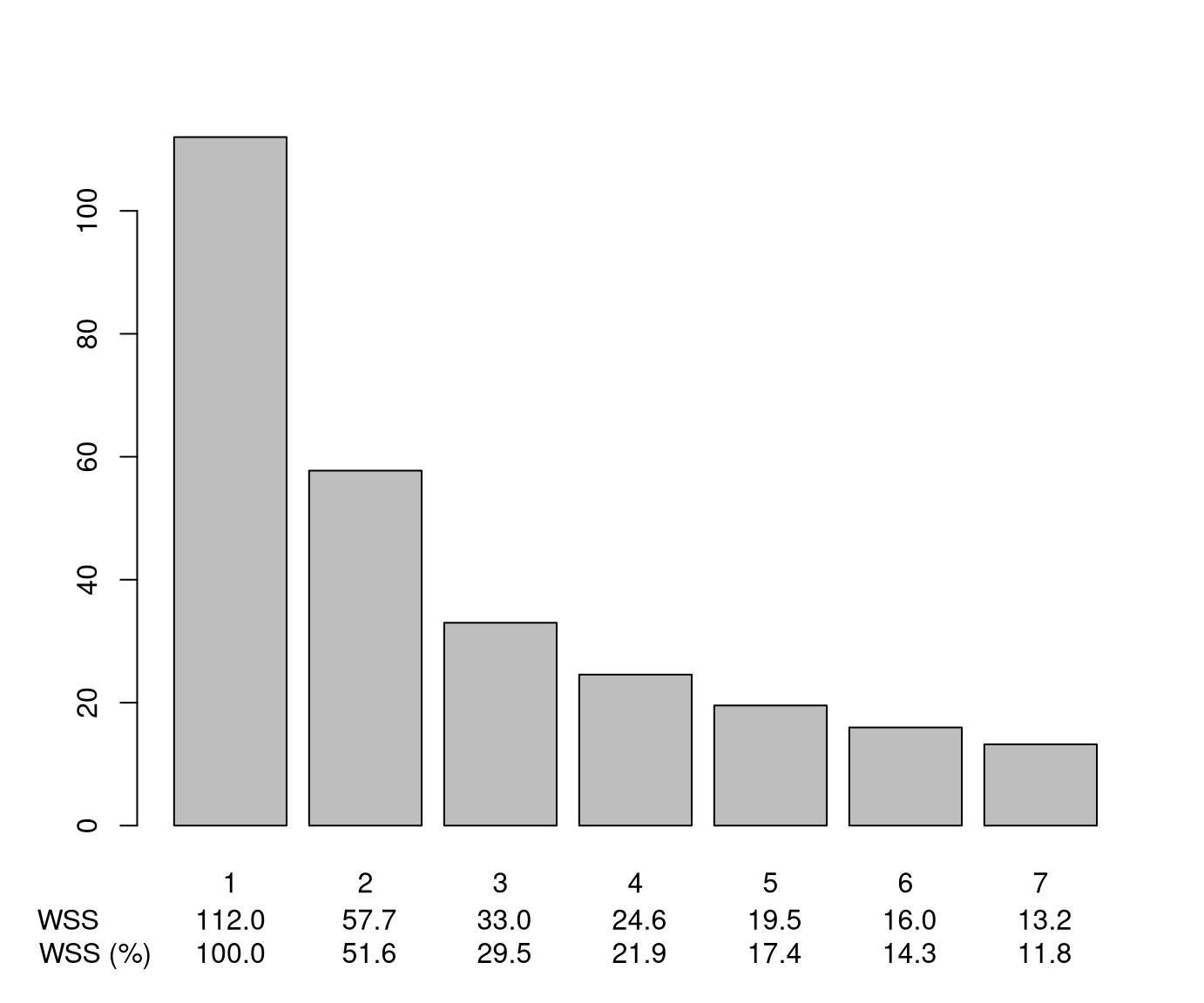
km7 = KMeans(n_clusters=7, init='random', n_init=50, random_state=22).fit(gsa)Then we collect the associated total within sum of squares and visualize them in a simple bar plot:
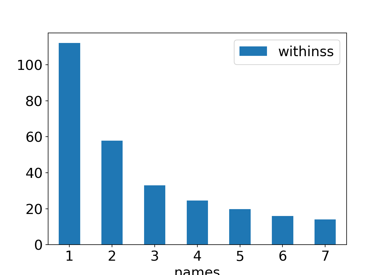
This shows that in relative terms the total within sum of squares drops to about a half for the 2-means solutions and less than a third for the 3-means solutions. For higher \(k\) the total within sum of squares drops only relatively little.
The relative changes compared to the total sum of squares can also be computed as:
Thus, a 3-means clustering appears to be sufficient here as changes for higher \(k\) are rather small.
8.6.3 Interpreting the clusters
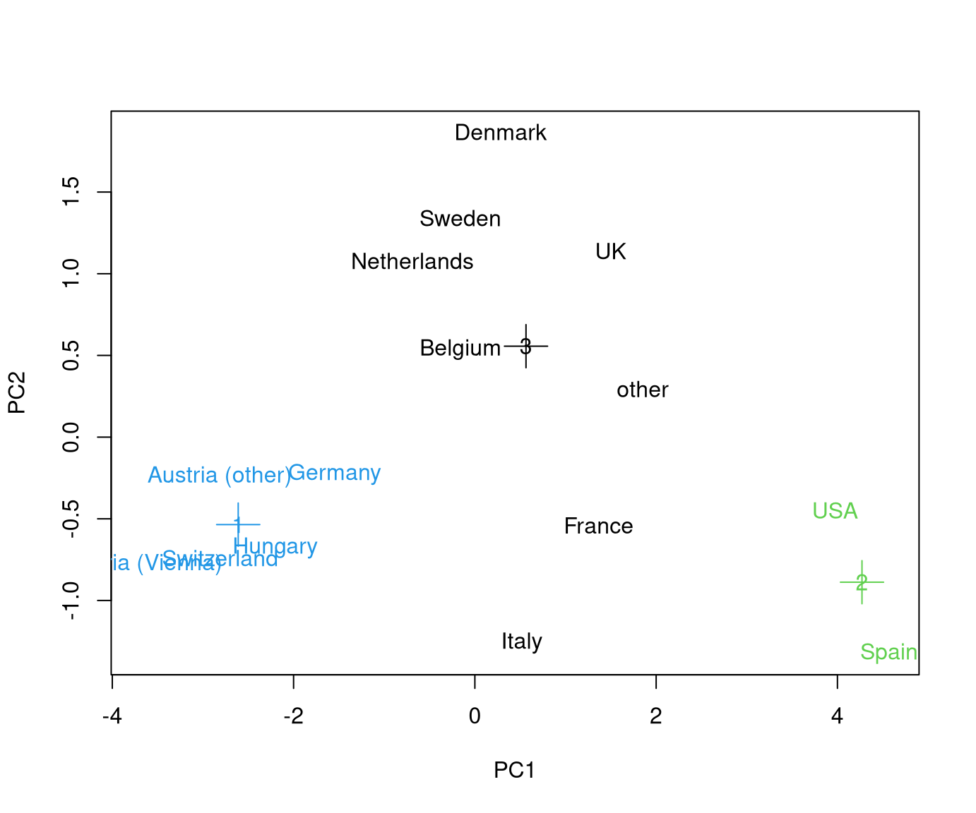
The 3-means result in fact yields the same clusters as the Hierarchical clustering in Chapter 7.
R
## Austria (Vienna)  Austria (other)          Belgium          Denmark           France
##                3                3                2                2                2
##          Germany          Hungary            Italy      Netherlands            Spain
##                3                3                2                2                1
##           Sweden      Switzerland               UK              USA            other
##                2                3                2                1                2
Python
gsa.reset_index(inplace=True);
gsa["Labels"] = km3.labels_
gsa.set_index(["Country", "Labels"], inplace=True)

gsa
## SA01.tennis SA02.cycle ... SA19.sight SA21.museum
## Country Labels ...
## Austria (Vienna) 2 1.4187 1.3994 ... -1.3495 -0.8244
## Austria (other) 2 1.5783 1.6138 ... -1.0711 -0.7235
## Belgium 1 -0.6094 -0.1900 ... -0.5242 -0.5451
## Denmark 1 -0.1330 -0.5416 ... -0.1936 -0.6207
## France 1 -0.1526 -0.7144 ... 0.1639 0.3076
## Germany 2 -0.2285 0.8247 ... -0.5490 -0.5745
## Hungary 2 0.3238 0.8900 ... -0.0167 0.1558
## Italy 1 0.6322 0.1634 ... 0.3931 1.0689
## Netherlands 1 0.0794 0.6803 ... -0.5231 -0.6763
## Spain 0 -1.3853 -1.4897 ... 2.4629 2.5119
## Sweden 1 -0.7117 -0.6766 ... -0.1642 -0.7441
## Switzerland 2 1.8748 0.9287 ... -1.0749 -0.8807
## UK 1 -0.8036 -0.9762 ... 0.1964 -0.5013
## USA 0 -1.2259 -1.3534 ... 1.3937 1.2254
## other 1 -0.6573 -0.5584 ... 0.8563 0.8209
##
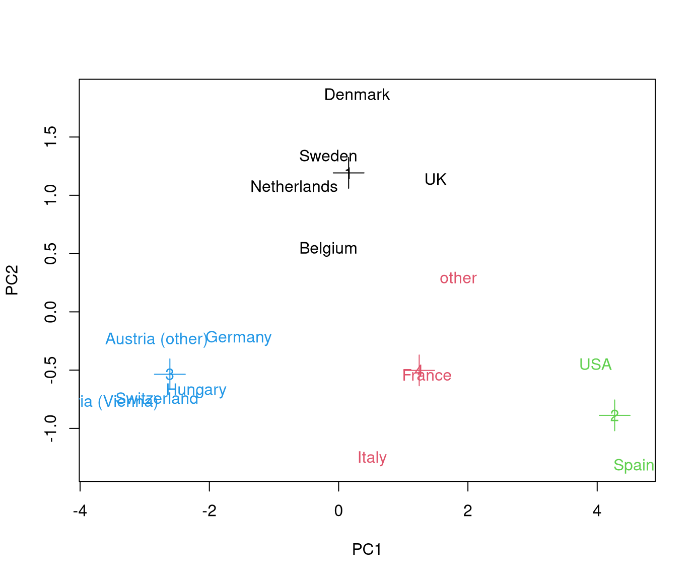
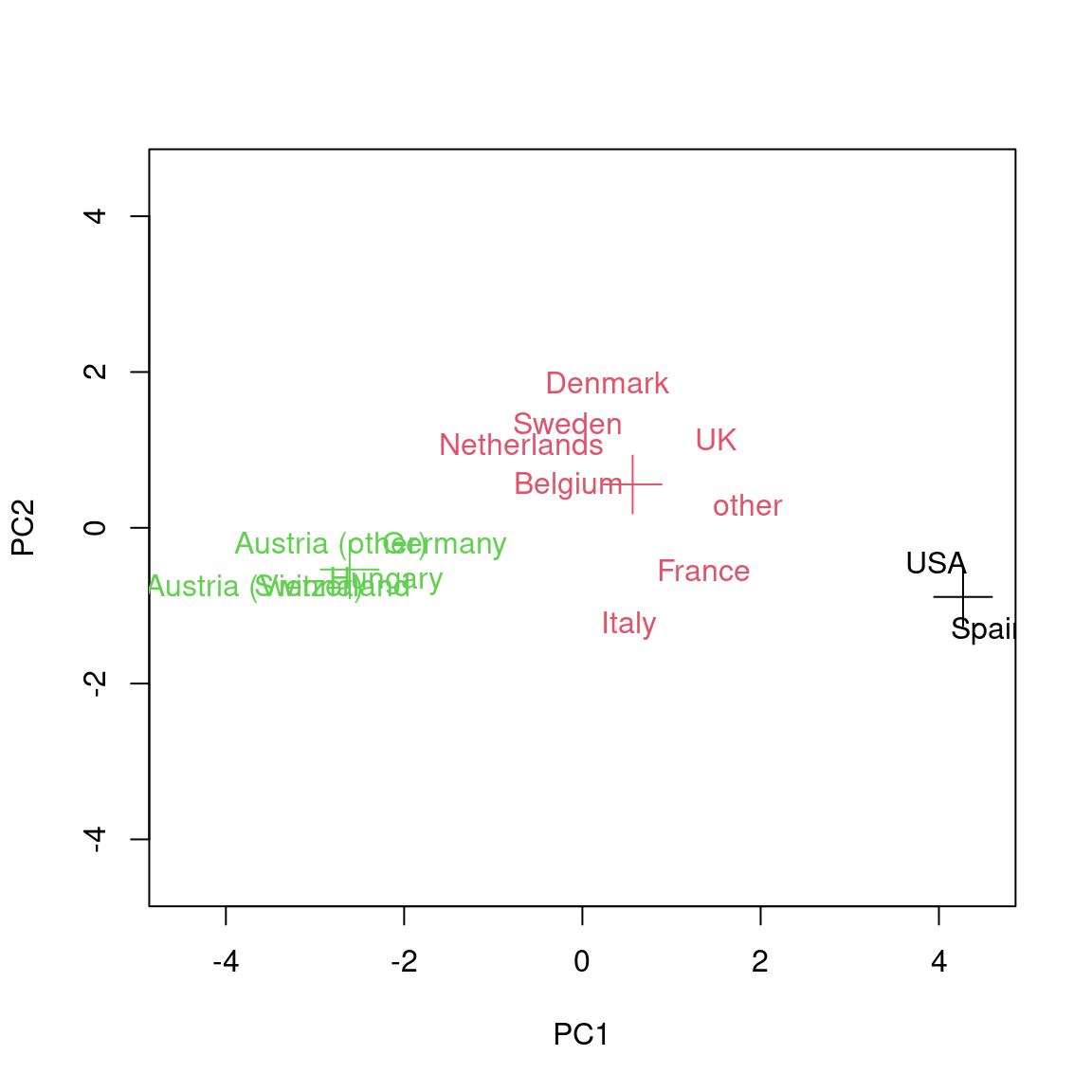
## [15 rows x 8 columns]Therefore, the same analysis of these clusters as in Chapter 7.5.3 could be carried out here. However, here we only point out one additional nice aspect: The color-coded plot of the first principal components shown in Chapter 7.5.3 can be complemented by a projection of the cluster means:
R
In R, by using the predict() method of prcomp objects.
gsa.pca <- prcomp(gsa, scale = TRUE)
plot(predict(gsa.pca)[,1:2], type = "n",
  xlim = c(-4.5, 4.5), ylim = c(-4.5, 4.5))
text(predict(gsa.pca)[,1:2], rownames(gsa), col = km3$cluster)
points(predict(gsa.pca, km3$centers)[,1:2], col = 1:3, pch = 3, cex = 3)
Python
gsa_pca = pca(n_components=8, normalize=False)
pca_results = gsa_pca.fit_transform(gsa.reset_index(drop=True))
## [pca] >Extracting column labels from dataframe.
## [pca] >Extracting row labels from dataframe.
## [pca] >The PCA reduction is performed on the [8] columns of the input dataframe.
## [pca] >Fit using PCA.
## [pca] >Compute loadings and PCs.
## [pca] >Compute explained variance.
## [pca] >Outlier detection using Hotelling T2 test with alpha=[0.05] and n_components=[8]
## [pca] >Multiple test correction applied for Hotelling T2 test: [fdr_bh]
## [pca] >Outlier detection using SPE/DmodX with n_std=[3]pc = gsa_pca.results['PC'].iloc[:, 0:2]
fig = plt.figure()
ax = plt.axis([-5.5, 5.5, -5.5, 5.5])
colors = plt.cm.get_cmap("rainbow", 3)## <string>:1: MatplotlibDeprecationWarning: The get_cmap function was deprecated in Matplotlib 3.7 and will be removed in 3.11. Use ``matplotlib.colormaps[name]`` or ``matplotlib.colormaps.get_cmap()`` or ``pyplot.get_cmap()`` instead.countries = gsa.index.levels[0]
for index, row in pc.iterrows():
color = colors(km3.labels_[index])
plt.text(row["PC1"], row["PC2"], countries[index], {"color": color})
print(km3.cluster_centers_)## [[-1.30558032 -1.42153324 -0.83328176 -1.85687623 1.18855647 1.61104305
## 1.92831865 1.86864579]
## [-0.29448778 -0.35169052 -0.5124076 -0.04426046 0.38495692 0.11731339
## 0.02556571 -0.11125325]
## [ 0.99341258 1.13131813 1.15316487 0.81356723 -1.09135367 -0.83211864
## -0.81223259 -0.56945311]]## [pca] >Column labels are auto-completed.
## [pca] >Outlier detection using Hotelling T2 test with alpha=[0.05] and n_components=[8]
## [pca] >Multiple test correction applied for Hotelling T2 test: [fdr_bh]
## [pca] >Outlier detection using SPE/DmodX with n_std=[3]for index in range(0, proj_cluster_means["PC1"].values.shape[0]):
m1 = proj_cluster_means["PC1"].values[index]
m2 = proj_cluster_means["PC2"].values[index]
plt.plot(m1, m2, color=colors(index), marker="+", markersize=16)
plt.xlabel("PC1")
plt.ylabel("PC2")
plt.show()
This shows that also in the projection on the first two principal components the cluster means are nicely in the center of their respective cluster.
To facilitate the creation of these plots, we took the code above, and made it slightly more flexible.
R
Additionally, in R we integrated it into a plot() method for kmeans
objects. Download the plot.kmeans.R
file in your working directory.
Our plot() method for kmeans objects requires two arguments: the fitted kmeans() output and the corresponding original data (in our case the scaled Guest Survey Austria data).
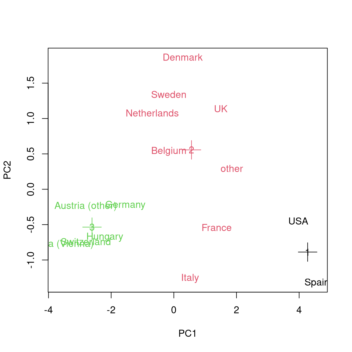
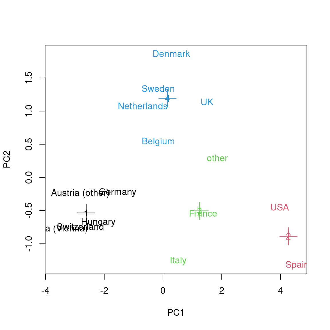
Using this function we can easily compare the optimal 3-means to the optimal
4-means result:
Python
def plot_kmeans(km, data):
"""
@ToDo
"""
gsa_pca = pca(n_components=None, normalize=False)
pca_results = gsa_pca.fit_transform(data.iloc[:, 2:])
pc = gsa_pca.results['PC'].iloc[:, 0:2]
n_clusters = km.get_params()["n_clusters"]
fig = plt.figure()
plt.axis([-5.5, 5.5, -5.5, 5.5])
colors = plt.cm.get_cmap("rainbow", n_clusters)
for index, row in pc.iterrows():
color = colors(km.labels_[index])
plt.text(row["PC1"], row["PC2"], data["Country"][index], {"color": color})
proj_cluster_means = gsa_pca.transform(np.array(km.cluster_centers_))
for index in range(0, n_clusters):
m1 = proj_cluster_means["PC1"].values[index]
m2 = proj_cluster_means["PC2"].values[index]
plt.plot(m1, m2, color=colors(index), marker="+", markersize=16)
plt.xlabel("PC1")
plt.ylabel("PC2")
plt.show()## [pca] >n_components is set to 7
## [pca] >Extracting column labels from dataframe.
## [pca] >Extracting row labels from dataframe.
## [pca] >The PCA reduction is performed on the [8] columns of the input dataframe.
## [pca] >Fit using PCA.
## [pca] >Compute loadings and PCs.
## [pca] >Compute explained variance.
## [pca] >Outlier detection using Hotelling T2 test with alpha=[0.05] and n_components=[7]
## [pca] >Multiple test correction applied for Hotelling T2 test: [fdr_bh]
## [pca] >Outlier detection using SPE/DmodX with n_std=[3]
## <string>:13: MatplotlibDeprecationWarning: The get_cmap function was deprecated in Matplotlib 3.7 and will be removed in 3.11. Use ``matplotlib.colormaps[name]`` or ``matplotlib.colormaps.get_cmap()`` or ``pyplot.get_cmap()`` instead.
## [pca] >Column labels are auto-completed.
## [pca] >Outlier detection using Hotelling T2 test with alpha=[0.05] and n_components=[7]
## [pca] >Multiple test correction applied for Hotelling T2 test: [fdr_bh]
## [pca] >Outlier detection using SPE/DmodX with n_std=[3]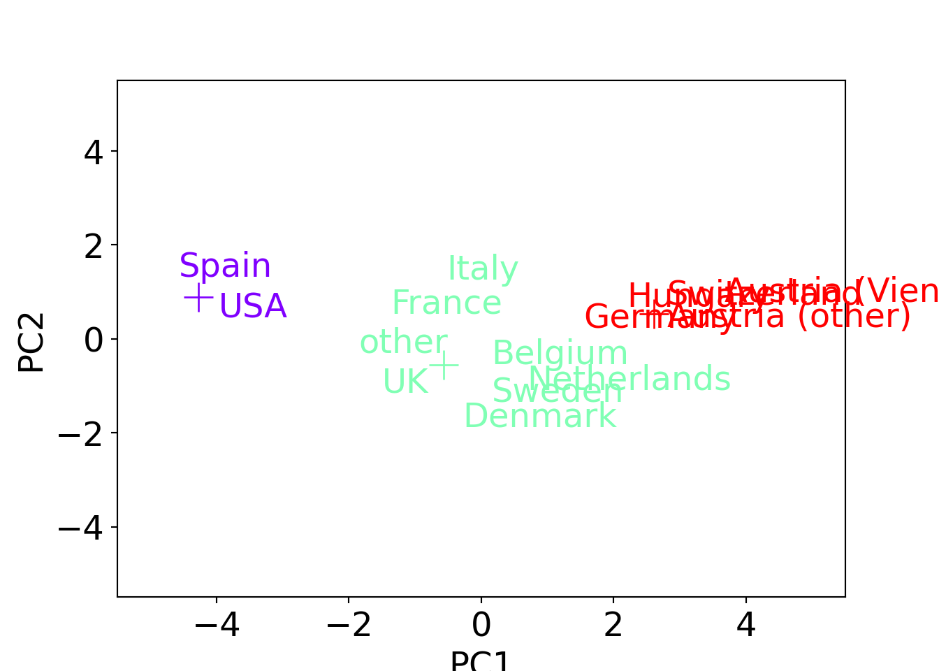
## [pca] >n_components is set to 7
## [pca] >Extracting column labels from dataframe.
## [pca] >Extracting row labels from dataframe.
## [pca] >The PCA reduction is performed on the [8] columns of the input dataframe.
## [pca] >Fit using PCA.
## [pca] >Compute loadings and PCs.
## [pca] >Compute explained variance.
## [pca] >Outlier detection using Hotelling T2 test with alpha=[0.05] and n_components=[7]
## [pca] >Multiple test correction applied for Hotelling T2 test: [fdr_bh]
## [pca] >Outlier detection using SPE/DmodX with n_std=[3]
## <string>:13: MatplotlibDeprecationWarning: The get_cmap function was deprecated in Matplotlib 3.7 and will be removed in 3.11. Use ``matplotlib.colormaps[name]`` or ``matplotlib.colormaps.get_cmap()`` or ``pyplot.get_cmap()`` instead.
## [pca] >Column labels are auto-completed.
## [pca] >Outlier detection using Hotelling T2 test with alpha=[0.05] and n_components=[7]
## [pca] >Multiple test correction applied for Hotelling T2 test: [fdr_bh]
## [pca] >Outlier detection using SPE/DmodX with n_std=[3]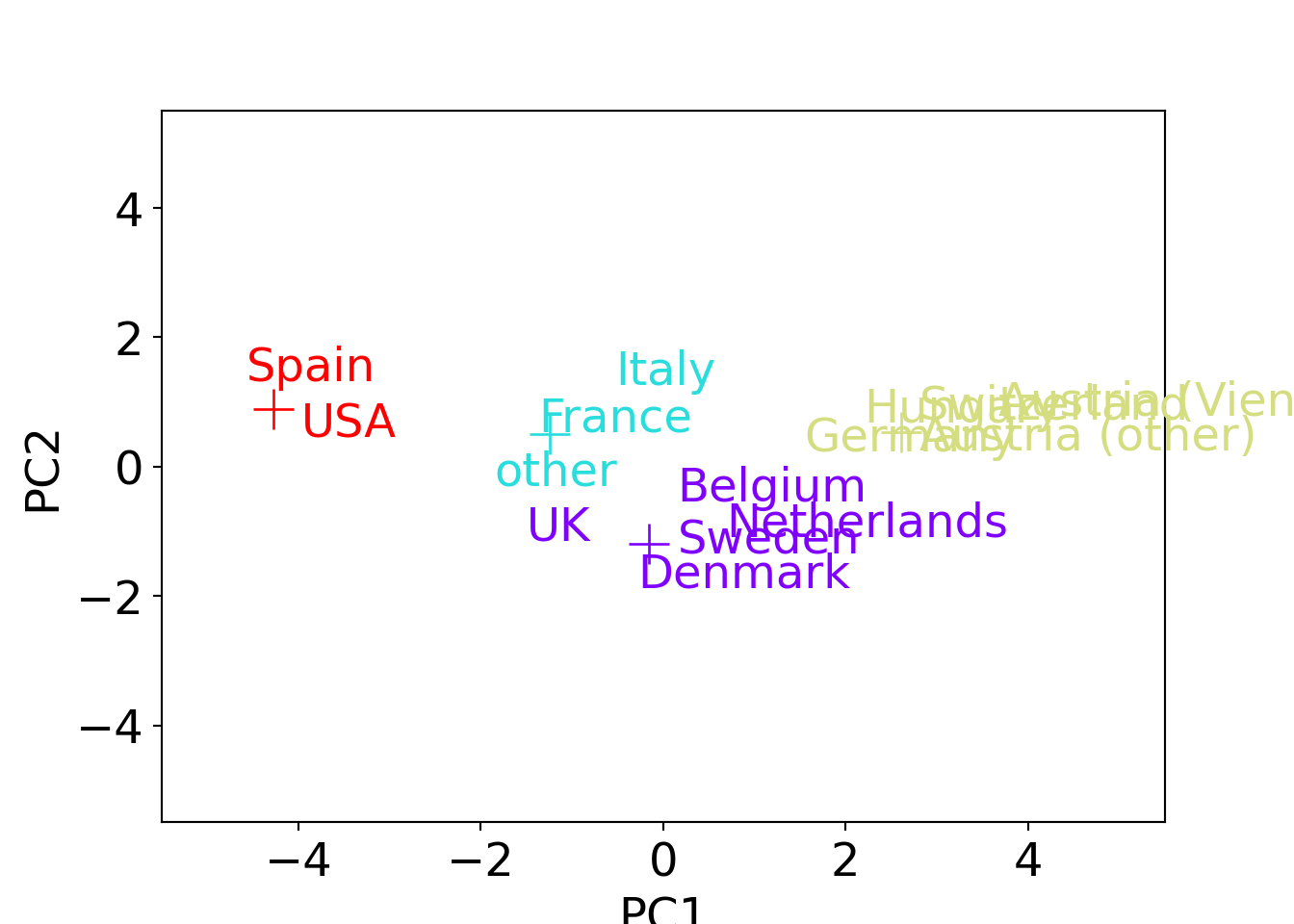
Up to the cluster assignment of the “other” country level, this is again essentially what hierarchical clustering yielded. The corresponding means of the scaled data are:
R
## SA01.tennis SA02.cycle SA03.ride SA05.swim SA17.shop SA18.concert SA19.sight
## 1 -1.305580 -1.421533 -0.833282 -1.8568762 1.188556 1.611043 1.9283186
## 2 -0.294488 -0.351691 -0.512408 -0.0442605 0.384957 0.117313 0.0255657
## 3 0.993413 1.131318 1.153165 0.8135672 -1.091354 -0.832119 -0.8122326
## SA21.museum
## 1 1.868646
## 2 -0.111253
## 3 -0.569453## SA01.tennis SA02.cycle SA03.ride SA05.swim SA17.shop SA18.concert SA19.sight
## 1 0.9934126 1.131318 1.153165 0.813567 -1.091354 -0.832119 -0.812233
## 2 -1.3055803 -1.421533 -0.833282 -1.856876 1.188556 1.611043 1.928319
## 3 -0.0592015 -0.369766 -0.448494 -0.386373 0.177842 0.909215 0.471104
## 4 -0.4356596 -0.340845 -0.550756 0.161007 0.509226 -0.357827 -0.241757
## SA21.museum
## 1 -0.569453
## 2 1.868646
## 3 0.732482
## 4 -0.617494Python
## [[-1.30558032 -1.42153324 -0.83328176 -1.85687623  1.18855647  1.61104305
##    1.92831865  1.86864579]
##  [-0.29448778 -0.35169052 -0.5124076  -0.04426046  0.38495692  0.11731339
##    0.02556571 -0.11125325]
##  [ 0.99341258  1.13131813  1.15316487  0.81356723 -1.09135367 -0.83211864
## -0.81223259 -0.56945311]]## [[-0.43565956 -0.3408453 -0.55075583 0.16100713 0.50922588 -0.35782735
## -0.24175749 -0.61749425]
## [-0.05920148 -0.36976589 -0.44849388 -0.3863731 0.177842 0.90921461
## 0.47110438 0.73248174]
## [ 0.99341258 1.13131813 1.15316487 0.81356723 -1.09135367 -0.83211864
## -0.81223259 -0.56945311]
## [-1.30558032 -1.42153324 -0.83328176 -1.85687623 1.18855647 1.61104305
## 1.92831865 1.86864579]]