Chapter 13 Linear Regression
In Part I: Dependencies between \(p\) variables \(X_1, \dots, X_p\), where all variables are considered equally. Of interest: Joint multivariate distribution of all variables.
In Part II: Dependencies between 2 variables \(Y\) and \(X\), where the two variables could either be considered equally or for \(Y\) given \(X\).
In Part III: Modeling the dependent (or response) variable \(Y\) conditional on explanatory variables \(X_1, \dots, X_k\). Thus, the variables are not considered equally but only the explanation/prediction of \(Y\) given the variables \(X_1, \dots, X_k\) is of interest.
Idea: The dependent quantitative variable \(Y\) can be modeled as a linear function of the \(k\) explanatory variables (or regressors) \(X_1, \dots, X_k\). The first regressor is typically a constant (or intercept) \(X_1 = 1\).
Notation: The data is a sample of \(n\) observations of the dependent variable \(y_i\) and a regressor vector \(x_i = (1, x_{i2}, \dots, x_{ik})^\top\) (\(i = 1, \dots, n\)).
Model equation: \(y_i\) is assumed to be a linear function of the regressors \(x_{ij}\) (with slope coefficients \(\beta_j\)) plus a random error or disturbance term \(\varepsilon_i\).
\[\begin{eqnarray*} y_i & = & \beta_1 ~+~ \beta_2 \cdot x_{i2} ~+~ \dots ~+~ \beta_k \cdot x_{ik} ~+~ \varepsilon_i \\ & = & x_i^\top \beta ~+~ \varepsilon_i \end{eqnarray*}\] Fundamental assumption: The errors have a zero mean, i.e., \(\text{E}(\varepsilon_i) = 0\).
Thus: The linear function captures the expectation of \(Y_i\).
\[\begin{equation*} \text{E}(Y_i) ~=~ \mu_i ~=~ x_i^\top \beta. \end{equation*}\]
Moreover: In many situations not only the error term \(\varepsilon_i\) (and thus the dependent variable \(Y_i\)) are stochastic but also the explanatory variables \(X_1, \dots, X_k\).
Of interest: Conditional expectation of \(Y_i\) given the \(X_j\).
\[\begin{equation*} \text{E}(Y_i ~|~ X_1 = x_{i1}, \dots, X_k = x_{ik}) ~=~ \beta_1 \cdot x_{i1} ~+~ \dots ~+~ \beta_k \cdot x_{ik} ~=~ x_i^\top \beta \end{equation*}\]
Interpretation: Emphasis that knowledge about the realizations of the regressors can be used for computing the expectation of the dependent variable.
In the following: As the setup with fixed non-stochastic regressors leads to virtually identical results as the conditional setup, the simpler notation without conditionals is used.
Matrix notation: Denote all \(n\) observations more compactly as
\[\begin{equation*} y ~=~ X \beta ~+~ \varepsilon, \end{equation*}\]
with
\[\begin{equation*} \begin{array}{lll} y = \left( \begin{array}{c} y_1 \\ y_2 \\ \vdots \\ y_n \end{array} \right), & X = \left( \begin{array}{llll} 1 & x_{12} & \ldots & x_{1k} \\ 1 & x_{22} & \ldots & x_{2k} \\ & & \vdots \\ 1 & x_{n2} & \ldots & x_{nk} \\ \end{array} \right), & \varepsilon = \left( \begin{array}{c} \varepsilon_1 \\ \varepsilon_2 \\ \vdots \\ \varepsilon_n \end{array} \right), \end{array} \end{equation*}\]
and \(\beta = (\beta_1, \dots, \beta_k)^\top\).
Thus: \(\text{E}(y) = X \beta\).
Interpretation of the coefficients:
\(\beta_1\) is the expectation of \(Y\) when all \(X_j\) (\(j \ge 2\)) are zero.
\(\beta_j\) (\(j \ge 2\)): The expectation of \(Y\) changes by \(\beta_j\), if \(X_j\) increases by one unit and all other \(X_\ell\) (\(\ell \neq j\)) remain fixed.
- For \(\beta_j > 0\): Positive association. \(Y\) increases on average, if \(X_j\) increases.
- For \(\beta_j < 0\): Negative association. \(Y\) decreases on average, if \(X_j\) increases.
- For \(\beta_j = 0\): No association. \(Y\) does not depend on \(X_j\).
Goal: Estimation of unknown coefficients \(\beta\), i.e., “learning” the model based on empirical observations for \(y_i\) and \(x_i\) (\(i = 1, \dots, n\)).
Prediction: Based on a coefficient estimate \(\hat \beta\) it is easy to obtain predictions \(\hat y_i\) for (potentially new) regressors \(x_i\).
\[\begin{eqnarray*} \hat y_i & = & \hat \beta_1 ~+~ \hat \beta_2 \cdot x_{i2} ~+~ \dots ~+~ \hat \beta_k \cdot x_{ik} \\ & = & x_i^\top \hat \beta \end{eqnarray*}\]
Prediction error: Deviations of observations \(y_i\) and predictions \(\hat y_i\) are called prediction errors or residuals.
\[\begin{equation*} \hat \varepsilon_i ~=~ y_i ~-~ \hat y_i \end{equation*}\]
Clear: Choose estimate \(\hat \beta\) so that prediction errors are as small as possible.
Question: What is as small as possible?
Answer: Minimize the residual sum of squares \(\mathit{RSS}(\beta)\) as a function of \(\beta\).
\[\begin{eqnarray*} \mathit{RSS}(\hat \beta) & = & \sum_{i = 1}^n \hat \varepsilon_i^2 ~=~ \sum_{i = 1}^n (y_i - \hat y_i)^2 \\ & = & \sum_{i = 1}^n (y_i - (\hat \beta_1 ~+~ \hat \beta_2 \cdot x_{i2} ~+~ \dots ~+~ \hat \beta_k \cdot x_{ik}))^2. \end{eqnarray*}\]
Jargon: The estimator \(\hat \beta\) that minimizes \(\mathit{RSS}(\beta)\) is called ordinary least-squares (OLS) estimator.
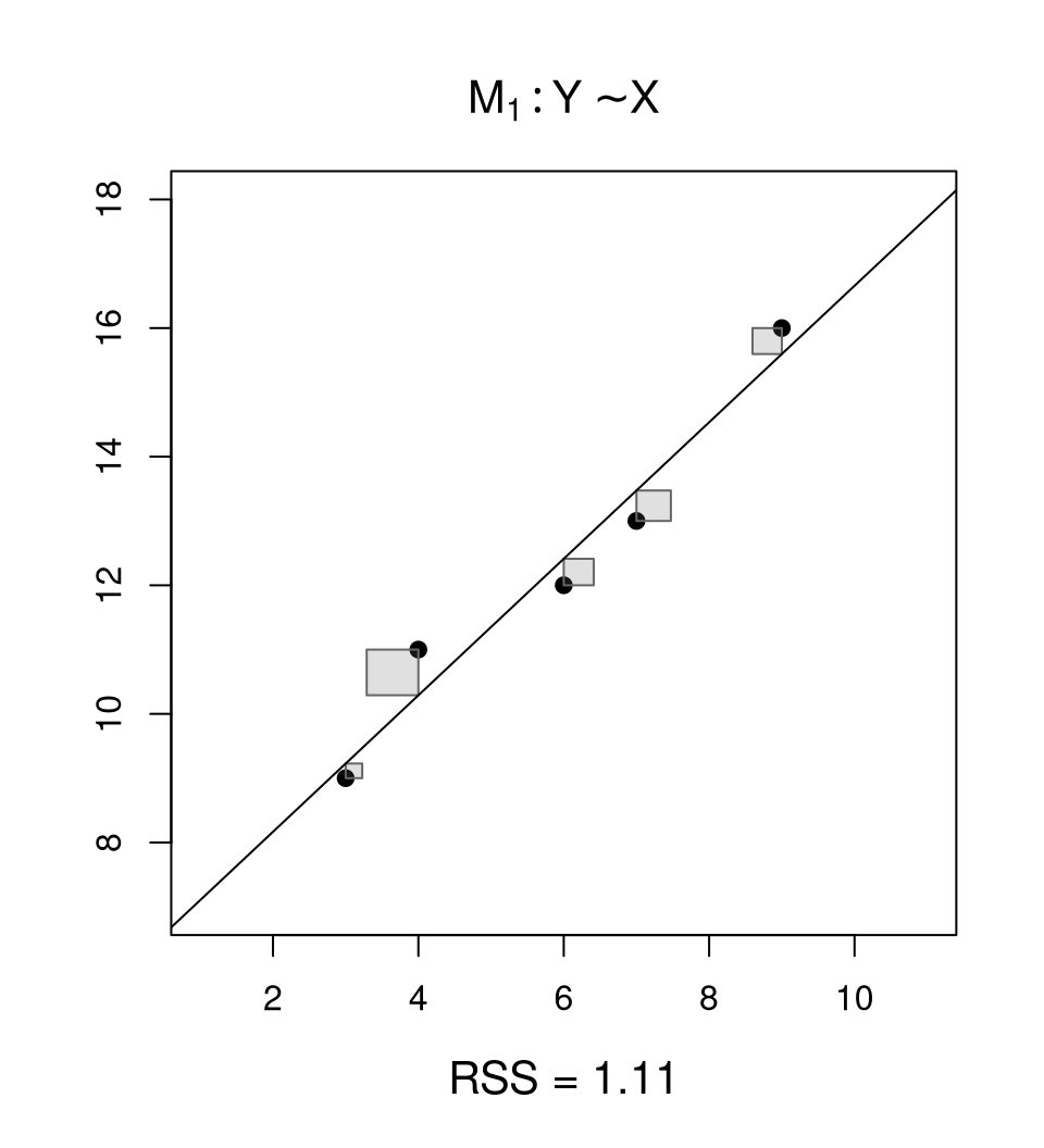
Example: Simple linear regression \(y_i = \beta_1 + \beta_2 \cdot x_i\) based on five observations.
##   x  y
## 1 3  9
## 2 6 12
## 3 7 13
## 4 9 16
## 5 4 11
Coefficients: OLS yields
##
## Call:
## lm(formula = y ~ x)
##
## Coefficients:
## (Intercept)            x
##      6.0439       1.0614
Prediction: For \(x_6 = 8\) we obtain \(\hat y_6 = 6.0439 + 1.0614 \cdot 8 = 14.535\).
13.1 Ordinary least squares
Analytically: Choose \(\hat \beta\) that minimizes \(\mathit{RSS}(\beta)\) (with the underlying \(y_i\) and \(x_i\) fixed to the observed data).
First order conditions: All partial derivatives of \(\mathit{RSS}(\beta)\) with respect to each \(\beta_j\) must be \(0\). This yields the so-called normal equations.
\[ X^\top X \beta ~=~ X^\top y \]
OLS estimator: If \(X^\top X\) is non-singular (see below) the normal equations can be solved explicitly.
\[ \hat \beta ~=~ (X^\top X)^{-1} X^\top y \]
Background: Using some algebra, the normal equations can be derived from the first order conditions as follows.
\[\begin{equation*} \begin{array}{lcll} \displaystyle \mathit{RSS}'(\beta) & = & 0 & \\ \displaystyle \left(\sum_{i = 1}^n (y_i - x_i^\top \beta)^2 \right)^\prime & = & 0 & \\ \displaystyle \sum_{i = 1}^n 2 \cdot (y_i - x_i^\top \beta) ~ (- x_{ij}) & = & 0 & \mbox{for all } j = 1, \dots, k \\ \displaystyle \sum_{i = 1}^n (y_i - x_i^\top \beta) ~ x_{ij} & = & 0 & \mbox{for all } j = 1, \dots, k \\ \displaystyle \sum_{i = 1}^n x_{ij} y_i & = & \displaystyle \sum_{i = 1}^n x_{ij} x_i^\top \beta & \mbox{for all } j = 1, \dots, k \\ \displaystyle X^\top y & = & \displaystyle X^\top X \beta & \end{array} \end{equation*}\]
Unbiasedness: If the errors \(\varepsilon_i\) indeed have zero expectation, then \(\hat \beta\) is unbiased. Thus, \(\text{E}(\hat \beta) = \beta\).
\[\begin{eqnarray*} \text{E}(\hat \beta) & = & \text{E}((X^\top X)^{-1} X^\top y) \\ & = & (X^\top X)^{-1} X^\top \text{E}(y) \\ & = & (X^\top X)^{-1} X^\top X \beta \\ & = & \beta \end{eqnarray*}\]
13.2 Inference: \(t\)-test and \(F\)-test
13.2.1 \(t\)-test
Inference: Assess whether \(Y\) depends at all on certain regressors \(X_j\).
\(t\)-test: For a single coefficient with hypotheses
\[\begin{equation*} H_0: ~ \beta_j ~=~ 0 ~\mbox{vs.}~ H_1: ~ \beta_j ~\neq~ 0. \end{equation*}\]
Alternatively: Decision between two nested models.
\[\begin{eqnarray*} &H_0: ~ Y ~=~ \beta_1 ~+~ \beta_2 \cdot X_2 ~+~ \dots ~{\phantom{+}~}~ \phantom{\beta_j \cdot X_j} ~{\phantom{+}~}~ \dots ~+~ \beta_k \cdot X_k ~+~ \varepsilon \\ &H_1: ~ Y ~=~ \beta_1 ~+~ \beta_2 \cdot X_2 ~+~ \dots ~+~ \beta_j \cdot X_j ~+~ \dots ~+~ \beta_k \cdot X_k ~+~ \varepsilon \end{eqnarray*}\]
\(t\)-statistic: Assess whether estimate \(\hat \beta_j\) is close to or far from zero, compared corresponding standard error.
\[ t ~=~ \frac{\hat \beta_j}{\widehat{\mathit{SD}(\hat \beta_j)}} \]
Typically: Derived under the assumptions that the error terms \(\varepsilon_i\) not only have zero mean but also equal variance \(\sigma^2\) (homoscedasticity).
\[\begin{eqnarray*} \mathit{SD}(\hat \beta_j) & = & \sqrt{\sigma^2 (X^\top X)_{jj}^{-1}} \\ \hat \sigma^2 & = & \frac{1}{n-k} \sum_{i = 1}^n (y_i - \hat y_i)^2 \\ \widehat{\mathit{SD}(\hat \beta_j)} & = & \sqrt{\hat \sigma^2 (X^\top X)_{jj}^{-1}} \end{eqnarray*}\]
Null distribution: Analogously to Chapter 9-12.
- Under the assumption of normally-distributed errors, the \(t\)-statistic is exactly \(t\)-distributed with \(n-k\) degrees of freedom.
- Asymptotically normally distributed (due to central limit theorem).
Critical values: The 2-sided critical values at significance level \(\alpha\) are \(\pm t_{n-k; 1 - \alpha/2}\), i.e., \(\pm\) the \((1 - \alpha/2)\) quantile of the \(t_{n-k}\) distribution. Rule of thumb: The critical values at the \(\alpha = 0.05\) level are approximately \(t_{n-k; 0.975} \approx 2\).
Test decision: Reject the null hypothesis if \(|t| > t_{n-k; 1 - \alpha/2}\).
\(p\)-value: Analogously compute the corresponding \(p\)-value \(p = \text{P}_{H_0}(|T| > |t|)\). Reject the null hypothesis if \(p < \alpha\).
Confidence interval: The level \(\alpha\) confidence interval for the true coefficient \(\beta_j\) can also be computed based on the critical values.
\[\begin{equation*} \left[ \hat \beta_j ~-~ t_{n-k; 1 - \alpha/2} \cdot \widehat{\mathit{SD}(\hat \beta_j)} ~;~~ \hat \beta_j ~+~ t_{n-k; 1 - \alpha/2} \cdot \widehat{\mathit{SD}(\hat \beta_j)} \right] \end{equation*}\]
Example: Simple linear regression based on five observations.
Summary table: Provides coefficient estimates \(\hat \beta_j\) with corresponding standard errors, \(t\)-statistics, and \(p\)-values.
##             Estimate Std. Error t value Pr(>|t|)
## (Intercept)    6.044      0.789    7.66   0.0046
## x              1.061      0.128    8.32   0.0036
Confidence intervals: At 5% significance level.
##              2.5 % 97.5 %
## (Intercept) 3.5336  8.554
## x           0.6553  1.468
13.2.2 \(F\)-test and analysis of variance
\(F\)-statistic: Assess whether the model under the alternative \(H_1\) with \(X_j\) fits equally well vs. much better than the model under the null hypothesis \(H_0\) without \(X_j\).
Coefficient estimates: \(\hat \beta\) is the unconstrained estimate under \(H_1\) vs. \(\widetilde \beta\) under \(H_0\) where \(\beta_j\) is constrained to zero.
Goodness of fit: Residual sums of squares, i.e., as optimized in the OLS estimation.
Clear: Constrained model under \(H_0\) is a special case of the unconstrained model under \(H_1\). Hence its residual sum of squares cannot be smaller.
\[\begin{equation*} \mathit{RSS}_0 ~=~ \mathit{RSS}(\widetilde \beta) ~\ge~ \mathit{RSS}(\hat \beta) ~=~ \mathit{RSS}_1 \end{equation*}\]
Example: Simple linear regression with vs. without regressor \(X\).
| \(H_0\): | \(\beta_1 = 0\), | Model \(M_0\): \(Y = \beta_0 + \varepsilon\) |
| \(H_1\): | \(\beta_1 \neq 0\), | Model \(M_1\): \(Y = \beta_0 + \beta_1 \cdot X + \varepsilon\) |
Coefficient estimates: \(\hat \beta\) in \(M_1\) vs. \(\widetilde \beta = (\overline y, 0)^\top\) in \(M_0\), i.e., the intercept is estimated by the empirical mean.
Goodness of fit: Corresponding residual sums of squares.
\[\begin{eqnarray*} RSS_{0} = \sum_{i = 1}^n (y_i - \overline y)^2, \quad RSS_{1} = \sum_{i = 1}^n (y_i - \hat y_i)^2 \end{eqnarray*}\]

Constrained model:
##
## Call:
## lm(formula = y ~ 1, data = dat)
##
## Coefficients:
## (Intercept)
##        12.2
Analysis of variance:
## Analysis of Variance Table
##
## Model 1: y ~ 1
## Model 2: y ~ x
##   Res.Df   RSS Df Sum of Sq    F Pr(>F)
## 1      4 26.80
## 2      3  1.11  1      25.7 69.2 0.0036
Again: The \(p\)-value from \(F\)-test and \(t\)-test of slope coefficient \(\beta_1\) is identical.
##   Estimate Std. Error t value Pr(>|t|)
## x    1.061      0.128    8.32   0.0036
Also: The \(F\)-statistic is the squared \(t\)-statistic \(t^2 = 8.32^2 = 69.2 = F\).
More generally: Analysis of variance can also assess nested models.
| \(H_0\): | Simpler (restricted) model |
| \(H_1\): | More complex (unrestricted) model |
Clear:
- The simpler model estimates \(\mathit{df}_0\) parameters, leading to \(\mathit{RSS}_0\) with \(n - \mathit{df}_0\) residual degrees of freedom.
- The more complex model estimates \(\mathit{df}_1 > \mathit{df}_0\) parameters, leading to \(\mathit{RSS}_1\) with \(n - \mathit{df}_1\) residual degrees of freedom.
- As the simpler model is a special case of (or nested in) the more complex model, its \(\mathit{RSS}_0\) cannot be smaller than \(\mathit{RSS}_1\).
\(F\)-statistic: Standardized difference of residual sums of squares.
\[\begin{equation*} F = \frac{ (\mathit{RSS}_0 - \mathit{RSS}_1) / (\mathit{df}_1-\mathit{df}_0)}{\mathit{RSS}_1/(n - \mathit{df}_1)}. \end{equation*}\]
Standardization: Based number of additional coefficients \(\mathit{df}_1 - \mathit{df}_0\) and residual variance under the alternative \(\hat \sigma^2 = \mathit{RSS}_1/(n - \mathit{df}_1)\).
Null distribution: Analogously to Chapter 9-12.
- Under the assumption of normally-distributed errors, the \(F\)-statistic is exactly \(F\)-distributed with \(\mathit{df}_1-\mathit{df}_0\) and \(n - \mathit{df}_1\) degrees of freedom.
- Asymptotically \(\chi_{\mathit{df}_1-\mathit{df}_0}^2\)-distributed with \(\mathit{df}_1-\mathit{df}_0\) degrees of freedom.
Res.Df |
RSS |
Df |
Sum of Sq |
F |
Pr(>F) |
|
|---|---|---|---|---|---|---|
1 |
\(n - \mathit{df}_0\) | \(\mathit{RSS}_0\) | ||||
2 |
\(n - \mathit{df}_1\) | \(\mathit{RSS}_1\) | \(\mathit{df}_1 - \mathit{df}_0\) | \(\mathit{RSS}_0-\mathit{RSS}_1\) | \(F\) | \(p\)-value |
Res.Df |
RSS |
Df |
Sum of Sq |
F |
Pr(>F) |
|
|---|---|---|---|---|---|---|
1 |
\(4\) | \(26.80\) | ||||
2 |
\(3\) | 1.11 | \(1\) | \(25.7\) | \(69.2\) | \(0.0036\) |
Coefficient of determination: Proportion of additional variance explained by the more complex model, i.e.,
\[\begin{eqnarray*} \frac{26.80 - 1.11}{26.80} ~=~ \frac{25.7}{26.80} ~=~ 0.96. \end{eqnarray*}\]
Moreover:
- The coefficient determination in comparison to the trivial intercept-only model is typically reported in model summary.
- Either: Proportion of explained variance in the corresponding ANOVA.
- Or equivalently: Squared correlation of response \(y_i\) and fitted values \(\hat y_i\).
- Hence known as \(R^2\) and always in \([0, 1]\).
\[\begin{eqnarray*} R^2 & = & \text{Cor}(y, \hat y)^2 \\ & = & \frac{\mathit{RSS}_0 ~-~ \mathit{RSS}_1}{\mathit{RSS}_0} \\ & = & 1 - \frac{\mathit{RSS}_1}{\mathit{RSS}_0} \\ \end{eqnarray*}\]
13.2.3 Summary
Example: Simple linear regression based on five observations. Compactly summarizes most quantities so far.
##
## Call:
## lm(formula = y ~ x)
##
## Residuals:
## 1 2 3 4 5
## -0.228 -0.412 -0.474 0.404 0.711
##
## Coefficients:
## Estimate Std. Error t value Pr(>|t|)
## (Intercept) 6.044 0.789 7.66 0.0046
## x 1.061 0.128 8.32 0.0036
##
## Residual standard error: 0.609 on 3 degrees of freedom
## Multiple R-squared: 0.958, Adjusted R-squared: 0.945
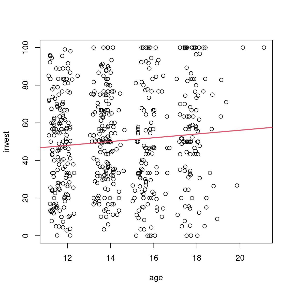
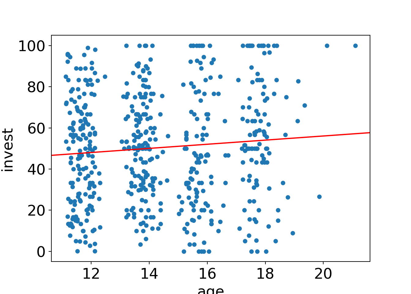
## F-statistic: 69.2 on 1 and 3 DF, p-value: 0.00364Example: Investment explained by age in myopic loss aversion (MLA) data. Replicates Pearson correlation test from Chapter 12.
##
## Call:
## lm(formula = invest ~ age, data = MLA)
##
## Residuals:
##    Min     1Q Median     3Q    Max
## -54.08 -20.67   0.08  20.20  51.09
##
## Coefficients:
##             Estimate Std. Error t value   Pr(>|t|)
## (Intercept)   35.998      7.064    5.10 0.00000047
## age            1.003      0.487    2.06       0.04
##
## Residual standard error: 26.7 on 568 degrees of freedom
## Multiple R-squared:  0.00743,    Adjusted R-squared:  0.00568
## F-statistic: 4.25 on 1 and 568 DF,  p-value: 0.0397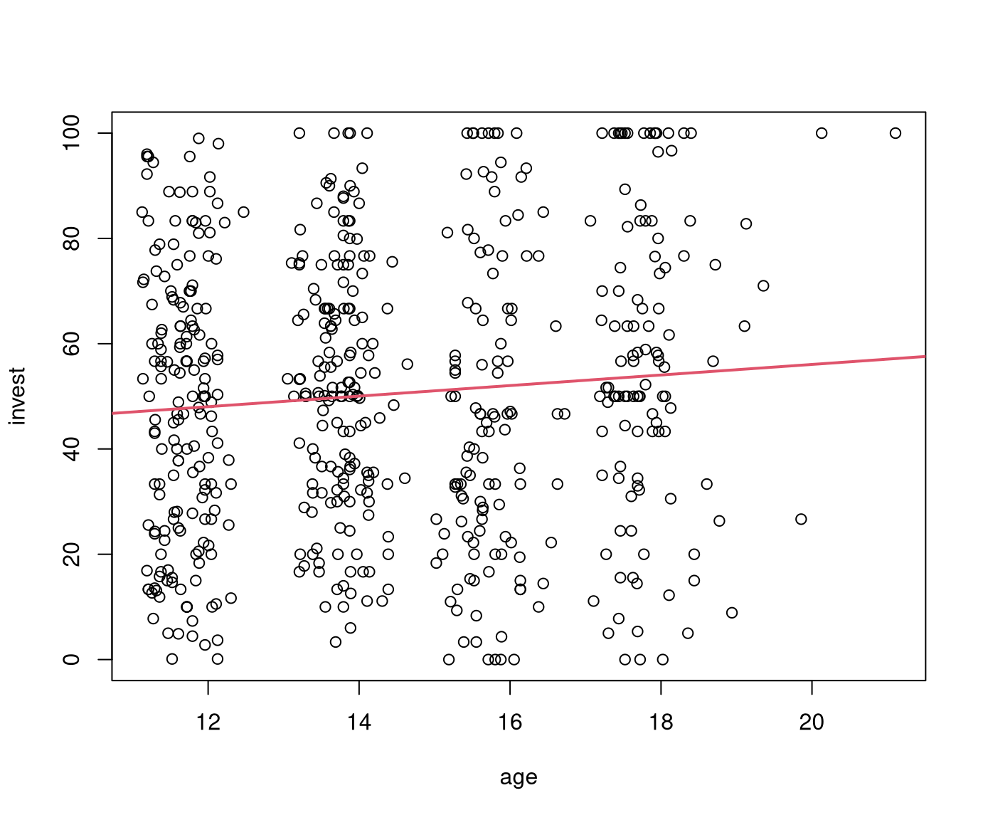
In Python:
##                             OLS Regression Results
## ==============================================================================
## Dep. Variable:                 invest   R-squared:                       0.007
## Model:                            OLS   Adj. R-squared:                  0.006
## Method:                 Least Squares   F-statistic:                     4.250
## Date:                Wed, 05 Mar 2025   Prob (F-statistic):             0.0397
## Time:                        14:23:06   Log-Likelihood:                -2680.8
## No. Observations:                 570   AIC:                             5366.
## Df Residuals:                     568   BIC:                             5374.
## Df Model:                           1
## Covariance Type:            nonrobust
## ==============================================================================
##                  coef    std err          t      P>|t|      [0.025      0.975]
## ------------------------------------------------------------------------------
## Intercept     35.9979      7.064      5.096      0.000      22.122      49.874
## age            1.0033      0.487      2.062      0.040       0.047       1.959
## ==============================================================================
## Omnibus:                       72.041   Durbin-Watson:                   1.395
## Prob(Omnibus):                  0.000   Jarque-Bera (JB):               19.687
## Skew:                           0.066   Prob(JB):                     5.31e-05
## Kurtosis:                       2.099   Cond. No.                         92.0
## ==============================================================================
##
## Notes:
## [1] Standard Errors assume that the covariance matrix of the errors is correctly specified.
13.3 Properties
Question: What are the properties of the OLS estimator? Under which assumptions does it lead to useful estimates?
Answer: Different assumptions about the error terms \(\varepsilon_i\) and regressors \(x_i\) are necessary for different properties, e.g.,
- The model with parameter \(\beta\) is well-defined.
- \(\hat \beta\) is a useful estimator for the true coefficients \(\beta\).
- \(\hat \beta\) is the best estimator for the true coefficients \(\beta\).
Assumptions:
- A1: Errors have (conditional) expectation zero: \(\text{E}(\varepsilon_i) = 0\).
- A2: Errors are homoscedastic with finite variance: \(\text{Var}(\varepsilon_i) = \sigma^2\).
- A3: Lack of correlation: \(\text{Cov}(\varepsilon_i,\varepsilon_j) = 0\).
- A4: Exogenous regressors: \(\text{Cov}(X_{ij},\varepsilon_i) = 0\).
- A5: No linear dependencies: \(\mathsf{rank}(X) = k\).
- A6: Normally-distributed errors: \(\varepsilon_i \sim \mathcal{N}(0,\sigma^2)\).
Gauss-Markov theorem: Under the assumptions A1 – A5 the OLS estimator \(\hat \beta\) is BLUE, the best linear unbiased estimator.
- Linear: \(\hat \beta\) is a linear combination of \(y_1,\dots, y_n\).
- Unbiased: \(\hat \beta\) has expectation \(\beta\).
- Best: \(\hat \beta\) is efficient among the linear unbiased estimators, i.e., all other estimators have greater variance (and thus lower precision).
Moreover: If A6 holds in addition, \(\hat \beta\) is efficient among all estimators.
Question: What happens if some assumptions are violated, in terms of point estimates \(\hat \beta_j\) and corresponding standard errors \(\widehat{\mathit{SD}(\hat \beta_j)}\) and inference?
Answer: Consequences of violated assumptions:
- None: \(\hat \beta\) is BLUE. Inference is valid exactly.
- A6: \(\hat \beta\) is still BLUE. Inference is valid approximately/asymptotically.
- A2/A3: \(\hat \beta\) is still unbiased but not efficient. Inference is biased as due to bias of the standard errors that would necessitate adjustment.
- A1: \(\hat \beta\) itself is biased. Model interpretations may not be meaningful at all.
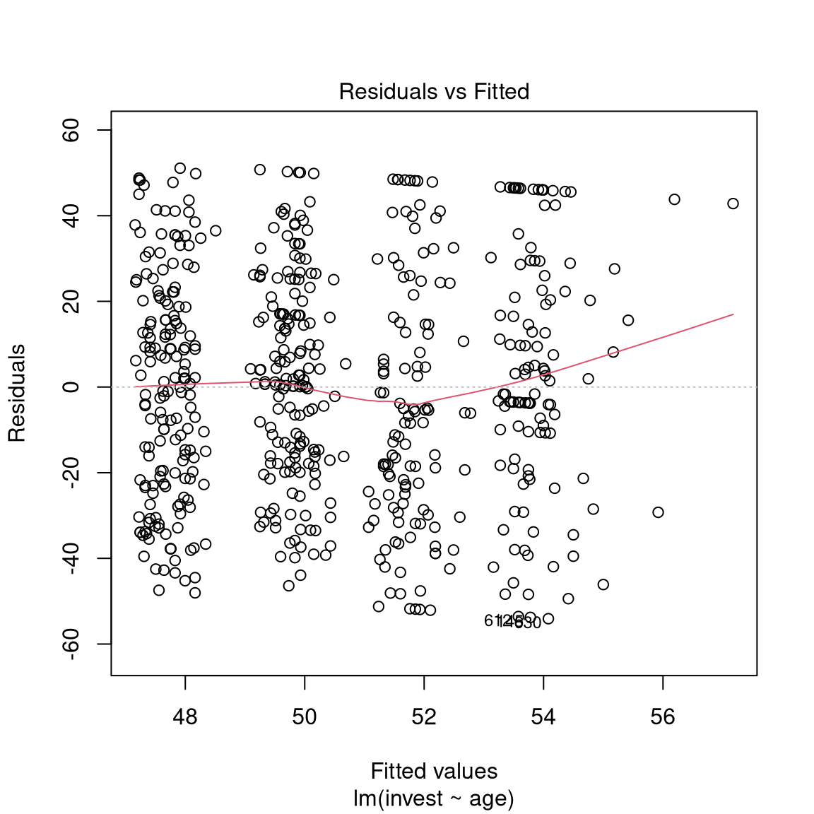
Examples: Violations of A1 (nonlinearity) and A2 (heteroscedasticity).
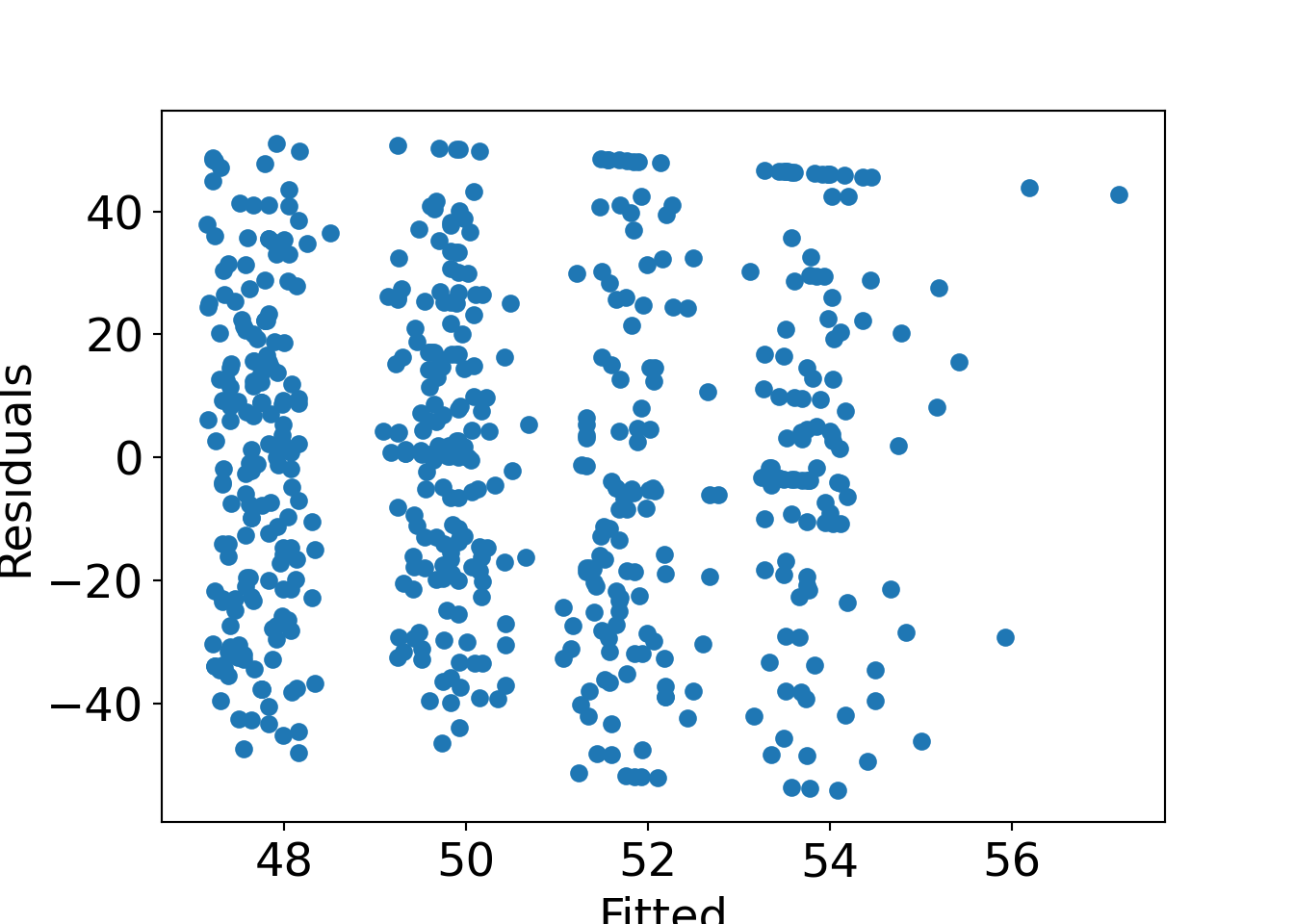
Diagnostic graphic: Residuals \(\hat \varepsilon_i\) vs. fitted values \(\hat y_i\).
13.3.1 Linearity
Question: Isn’t linearity a very strong assumption?
Answer: Yes and no. It is restrictive but also more flexible than obvious at first.
Remarks:
- Linearity just means linear in parameters \(\beta_1, \dots, \beta_k\) but not necessarily linear in the explanatory variables.
- Many models that are nonlinear in variables can be formulated as linear in parameters.
Examples: Simple examples for observation pairs \((x, y)\), i.e., a single regressor only. The index \(i\) and the error term \(\varepsilon_i\) are suppressed for simplicity.
Polynomial functions: Quadratic functions (and beyond).
\[\begin{equation*} y ~=~ \beta_1 ~+~ \beta_2 \cdot x ~+~ \beta_3 \cdot x^2. \end{equation*}\]
Exponential functions: Nominal growth rate \(\alpha_2\).
\[\begin{eqnarray*} y & = & \alpha_1 \cdot \mathsf{e}^{\alpha_2 \cdot x} \\ \log(y) & = & \log(\alpha_1) ~+~ \alpha_2 \cdot x \\ & = & \beta_1 ~+~ \beta_2 \cdot x. \end{eqnarray*}\]
Power functions: Elasticity \(\alpha_2\).
\[\begin{eqnarray*} y & = & \alpha_1 \cdot x^{\alpha_2} \\ \log(y) & = & \log(\alpha_1) ~+~ \alpha_2 \cdot \log(x) \\ & = & \beta_1 ~+~ \beta_2 \cdot \log(x). \end{eqnarray*}\]
13.3.2 Interpretation of parameters
Question: How can the coefficients in such model specifications be interpreted?
Intuitively:
- For variables “in levels”: Additive (i.e., absolute) changes are relevant.
- For variables “in logs”: Multiplicative (i.e., relative) changes are relevant.
Linear specification:
\[\begin{equation*} y ~=~ \beta_1 ~+~ \beta_2 \cdot x. \end{equation*}\]
Change in \(x\): An increase of \(x\) by one unit leads to the following \(\widetilde y\).
\[\begin{eqnarray*} \widetilde y & = & \beta_1 ~+~ \beta_2 \cdot (x+1) \\ & = & \beta_1 ~+~ \beta_2 \cdot x ~+~ \beta_2 \\ & = & y + \beta_2 \end{eqnarray*}\]
Thus: When \(x\) increases/decreases by one unit, the expectation of \(y\) increases/decreases absolutely by \(\beta_2\) units.
Semi-logarithmic specification:
\[\begin{equation*} \log(y) ~=~ \beta_1 ~+~ \beta_2 \cdot x. \end{equation*}\]
Change in \(x\): An increase of \(x\) by one unit leads to the following \(\widetilde y\).
\[\begin{eqnarray*} \log(\widetilde y) & = & \beta_1 ~+~ \beta_2 \cdot (x+1) \\ & = & \log(y) ~+~ \beta_2 \\ \widetilde y & = & y \cdot \exp(\beta_2) \\ & \approx & y \cdot (1 + \beta_2) \qquad \mbox{if $\beta_2$ small} \end{eqnarray*}\]
Thus: When \(x\) increases/decreases by one unit, the expectation of \(y\) increases/decreases relatively by a factor of \(\exp(\beta_2)\).
Rule of thumb: If \(\beta_2\) is small, this corresponds to a relative change by \(100\cdot\beta_2\)%.
Log-log specification:
\[\begin{equation*} \log(y) ~=~ \beta_1 ~+~ \beta_2 \cdot \log(x). \end{equation*}\]
Change in \(x\): An increase of \(x\) by one percent leads to the following \(\widetilde y\).
\[\begin{eqnarray*} \log(\widetilde y) & = & \beta_1 ~+~ \beta_2 \cdot \log(x \cdot 1.01) \\ & = & \beta_1 ~+~ \beta_2 \cdot \log(x) ~+~ \beta_2 \cdot \log(1.01) \\ & = & \log(y) ~+~ \beta_2 \cdot \log(1.01) \\ \widetilde y & = & y \cdot 1.01^{\beta_2} \\ % & \approx & y \cdot \exp(\beta_2 \cdot 0.01) \\ & \approx & y \cdot (1 + \beta_2/100) \qquad \mbox{if $\beta_2$ small} \end{eqnarray*}\]
Thus: When \(x\) increases/decreases by one percent, the expectation of \(y\) increases/decreases relatively by a factor of \(1.01^{\beta_2}\).
Rule of thumb: If \(\beta_2\) is small, this corresponds to a relative change by \(\beta_2\)%.
13.4 Model selection via significance tests
Question: With \(k-1\) explanatory variables \(X_2, \dots, X_k\) available, which should be included in the model?
Goal: The model should be made as simple as possible, but not simpler.
- Thus, use parameters parsimoniously.
- But also goodness of fit should not be significantly worse than more complex models.
- \(F\)-tests can assess trade-off between model complexity and goodness of fit.
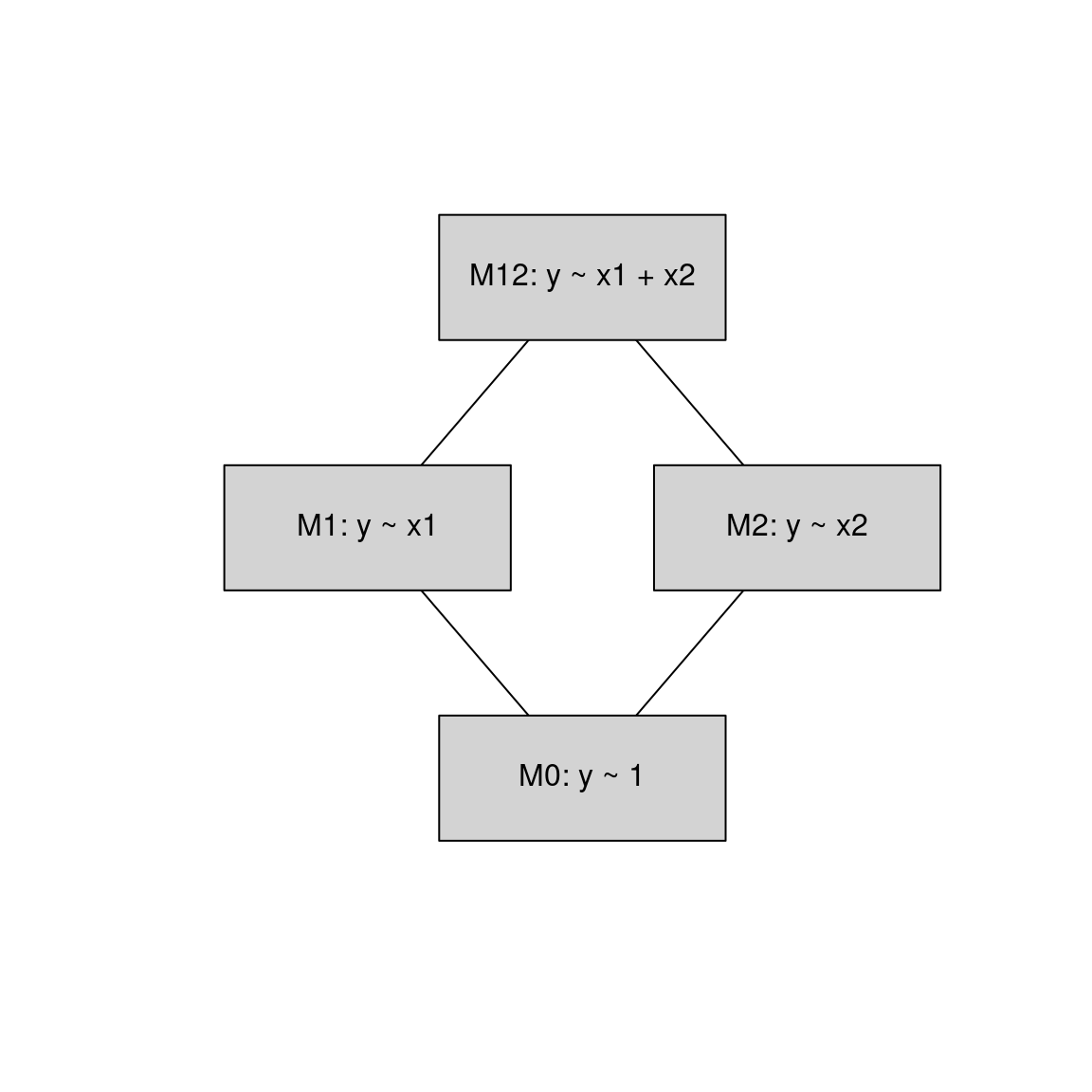
Example: With two explanatory variables \(X_1\) and \(X_2\) four nested models can be fitted.
\[\begin{equation*} \begin{array}{llcl} M_0: & Y & = & \beta_0 ~+~ \varepsilon \\ M_1: & Y & = & \beta_0 ~+~ \beta_1 \cdot X_{1} ~+~ \varepsilon \\ M_2: & Y & = & \beta_0 ~+~ \beta_2 \cdot X_{2} ~+~ \varepsilon \\ M_{12}: & Y & = & \beta_0 ~+~ \beta_1 \cdot X_{1} ~+~ \beta_2 \cdot X_{2} ~+~ \varepsilon \end{array} \end{equation*}\]
Backward selection:
- Start with the most complex model \(M_{12}\).
- Stepwise testing, dropping the most non-significant variable (if any).
- Stop when all remaining variables are significant.
Forward selection:
- Start with the simplest model \(M_{0}\).
- Stepwise testing, adding the most significant variable (if any).
- Stop when no more significant variables can be added.
Alternatively: Combine forward and backward selection starting from some initial model.
13.5 Tutorial
The myopic loss aversion (MLA) data (MLA.csv, MLA.rda) already analyzed in Chapter 12 are reconsidered. Rather than analyzing the dependence of invested point percentages (invest) on only a single explanatory variable at a time, the goal is to establish
a linear regression model encompassing all relevant explanatory variables simultaneously.
However, in this chapter only the dependence on the pupils’ age (age) is considered
before subsequent chapters will consider further explanatory variables and their
interactions.
13.5.1 Setup
Python
# Make sure that the required libraries are installed.
# Import the necessary libraries and classes:
import pandas as pd
import numpy as np
import matplotlib.pyplot as plt
import seaborn as sns
import statsmodels.api as sm
import statsmodels.formula.api as smf

pd.set_option("display.precision", 4) # Set display precision to 4 digits in pandas and numpy.
# Load dataset
MLA = pd.read_csv("MLA.csv", index_col=False, header=0)
# Select only 'invest' and 'age' which are used
MLA = MLA[["invest", "age"]]
# Preview the first 5 lines of the loaded data
MLA.head()## invest age
## 0 70.0000 11.7533
## 1 28.3333 12.0866
## 2 50.0000 11.7950
## 3 50.0000 13.7566
## 4 24.3333 11.295013.5.2 Model estimation
Equation:
\[ \begin{eqnarray*} y_i & = & \beta_1 ~+~ \beta_2 \cdot x_{i2} ~+~ \dots ~+~ \beta_k \cdot x_{ik} ~+~ \varepsilon_i \\ & = & x_i^\top \beta ~+~ \varepsilon_i \end{eqnarray*} \]
Matrix notation: \[ y ~=~ X \beta ~+~ \varepsilon \]
Ordinary least squares (OLS) estimator: \[ \hat \beta ~=~ (X^\top X)^{-1} X^\top y \]
Main function (linear model):
R
Main function: lm().
##
## Call:
## lm(formula = invest ~ age, data = MLA)
##
## Coefficients:
## (Intercept)          age
##          36            1
Python
Main function: smf.ols() (ordinary least squares).
##                             OLS Regression Results
## ==============================================================================
## Dep. Variable:                 invest   R-squared:                       0.007
## Model:                            OLS   Adj. R-squared:                  0.006
## Method:                 Least Squares   F-statistic:                     4.250
## Date:                Wed, 05 Mar 2025   Prob (F-statistic):             0.0397
## Time:                        14:23:07   Log-Likelihood:                -2680.8
## No. Observations:                 570   AIC:                             5366.
## Df Residuals:                     568   BIC:                             5374.
## Df Model:                           1
## Covariance Type:            nonrobust
## ==============================================================================
##                  coef    std err          t      P>|t|      [0.025      0.975]
## ------------------------------------------------------------------------------
## Intercept     35.9979      7.064      5.096      0.000      22.122      49.874
## age            1.0033      0.487      2.062      0.040       0.047       1.959
## ==============================================================================
## Omnibus:                       72.041   Durbin-Watson:                   1.395
## Prob(Omnibus):                  0.000   Jarque-Bera (JB):               19.687
## Skew:                           0.066   Prob(JB):                     5.31e-05
## Kurtosis:                       2.099   Cond. No.                         92.0
## ==============================================================================
##
## Notes:
## [1] Standard Errors assume that the covariance matrix of the errors is correctly specified.
13.5.3 Predictions
New data:
Obtain predictions:
13.5.4 Inference
Standard regression summary output with marginal \(t\)-tests:
R
##
## Call:
## lm(formula = invest ~ age, data = MLA)
##
## Residuals:
##    Min     1Q Median     3Q    Max
## -54.08 -20.67   0.08  20.20  51.09
##
## Coefficients:
##             Estimate Std. Error t value   Pr(>|t|)
## (Intercept)   35.998      7.064    5.10 0.00000047
## age            1.003      0.487    2.06       0.04
##
## Residual standard error: 26.7 on 568 degrees of freedom
## Multiple R-squared:  0.00743,    Adjusted R-squared:  0.00568
## F-statistic: 4.25 on 1 and 568 DF,  p-value: 0.0397
Python
##                             OLS Regression Results
## ==============================================================================
## Dep. Variable:                 invest   R-squared:                       0.007
## Model:                            OLS   Adj. R-squared:                  0.006
## Method:                 Least Squares   F-statistic:                     4.250
## Date:                Wed, 05 Mar 2025   Prob (F-statistic):             0.0397
## Time:                        14:23:09   Log-Likelihood:                -2680.8
## No. Observations:                 570   AIC:                             5366.
## Df Residuals:                     568   BIC:                             5374.
## Df Model:                           1
## Covariance Type:            nonrobust
## ==============================================================================
##                  coef    std err          t      P>|t|      [0.025      0.975]
## ------------------------------------------------------------------------------
## Intercept     35.9979      7.064      5.096      0.000      22.122      49.874
## age            1.0033      0.487      2.062      0.040       0.047       1.959
## ==============================================================================
## Omnibus:                       72.041   Durbin-Watson:                   1.395
## Prob(Omnibus):                  0.000   Jarque-Bera (JB):               19.687
## Skew:                           0.066   Prob(JB):                     5.31e-05
## Kurtosis:                       2.099   Cond. No.                         92.0
## ==============================================================================
##
## Notes:
## [1] Standard Errors assume that the covariance matrix of the errors is correctly specified.
Corresponding confidence intervals:
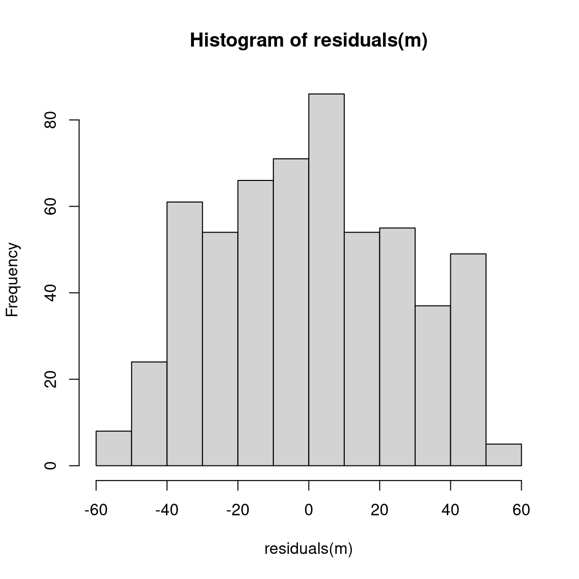
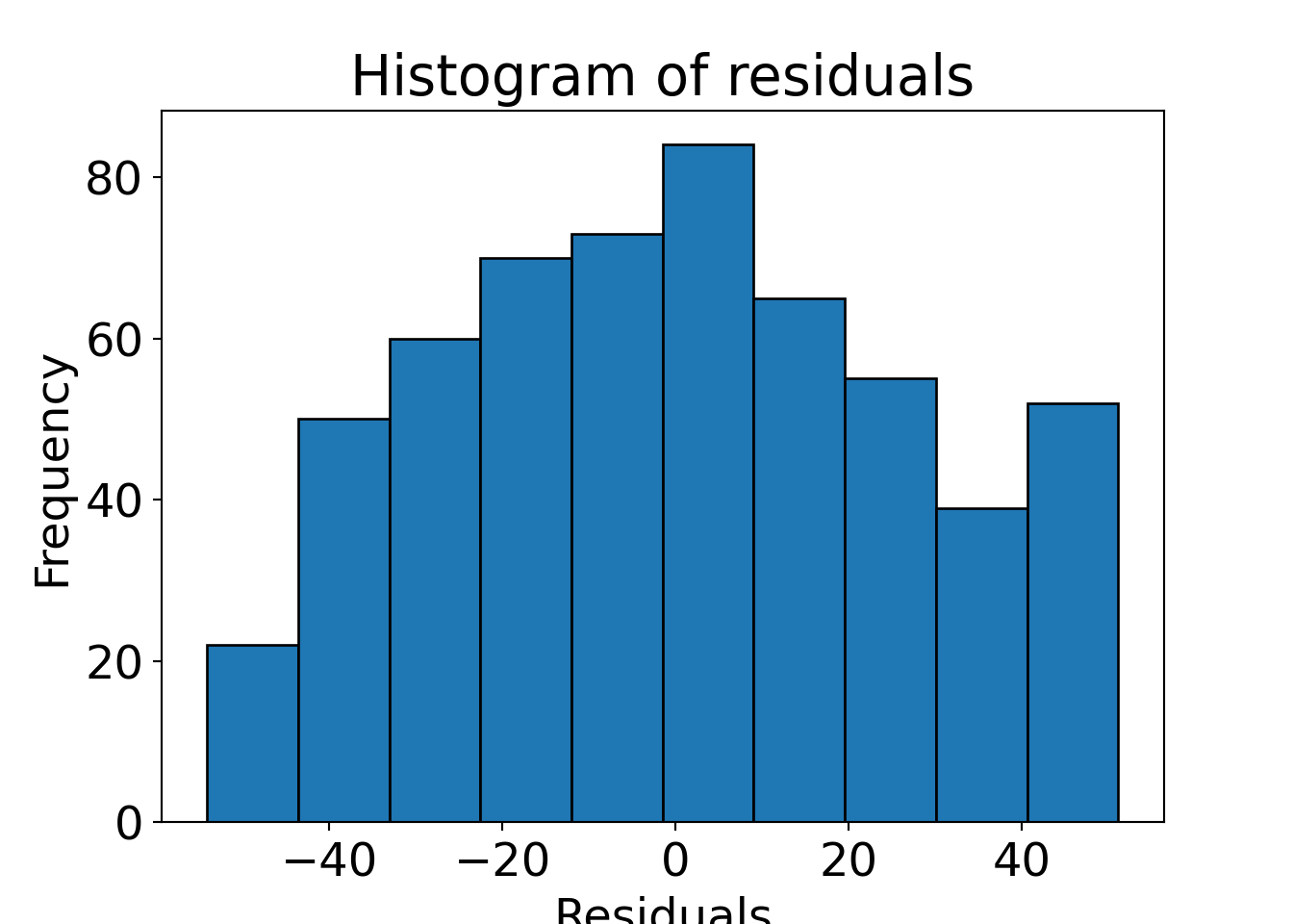
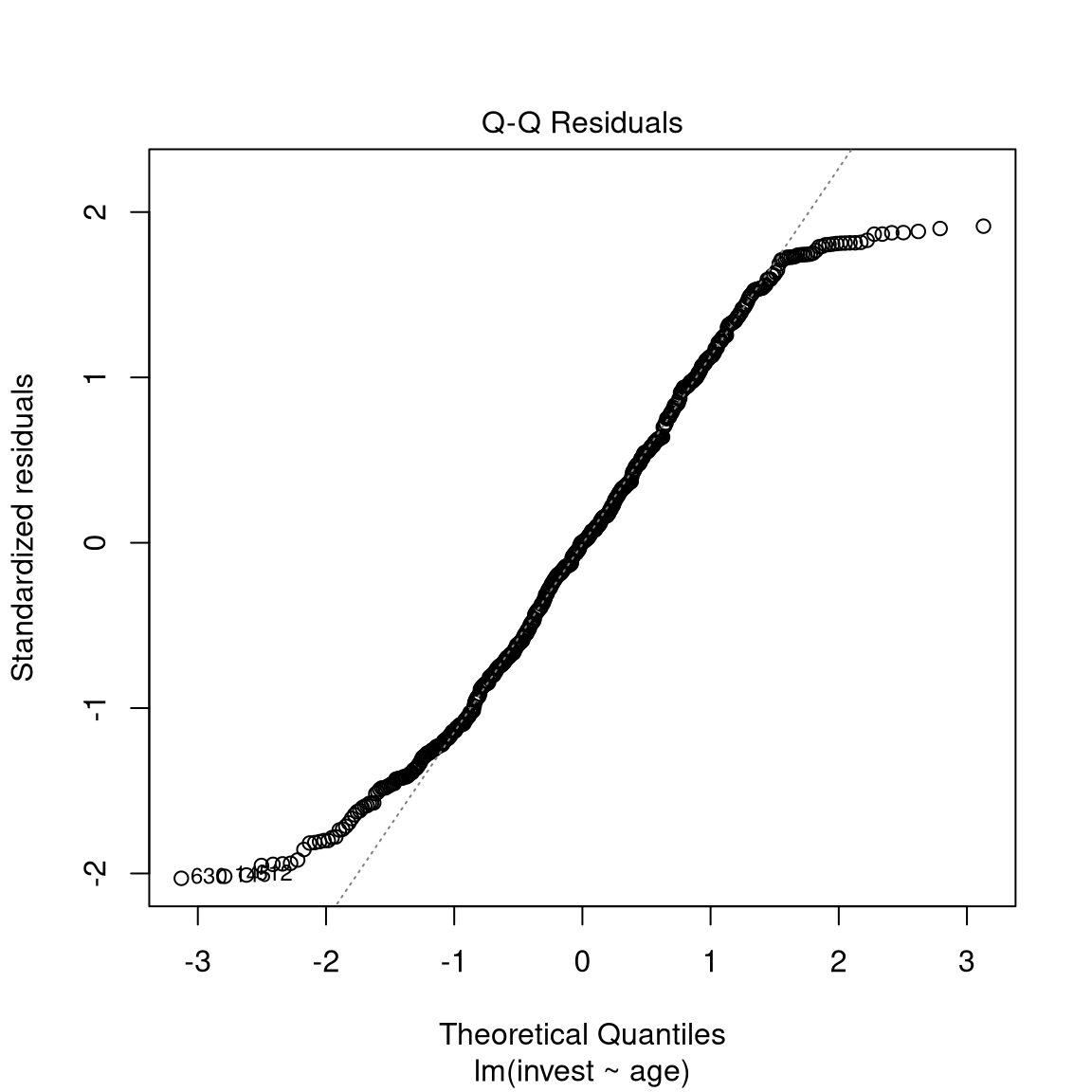
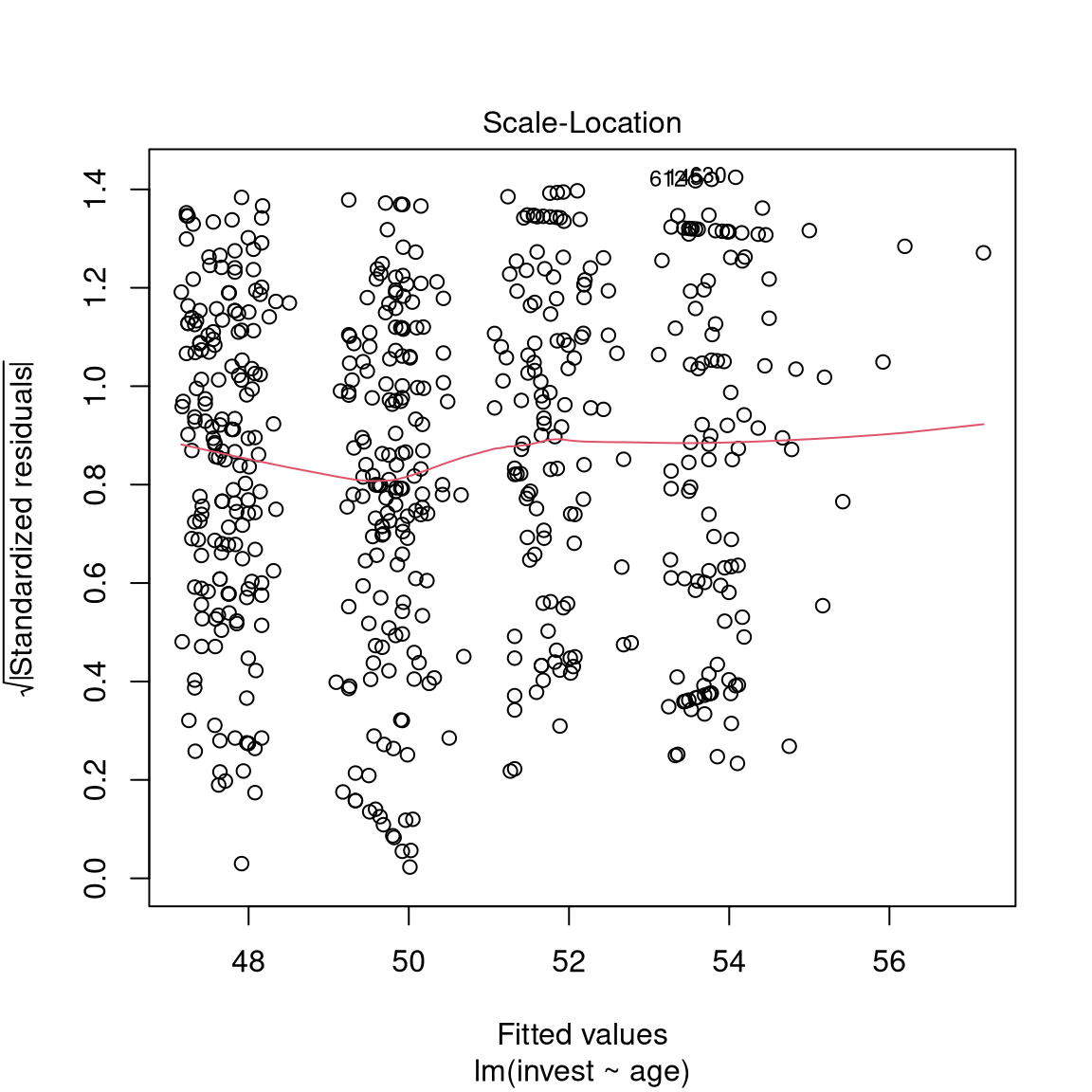
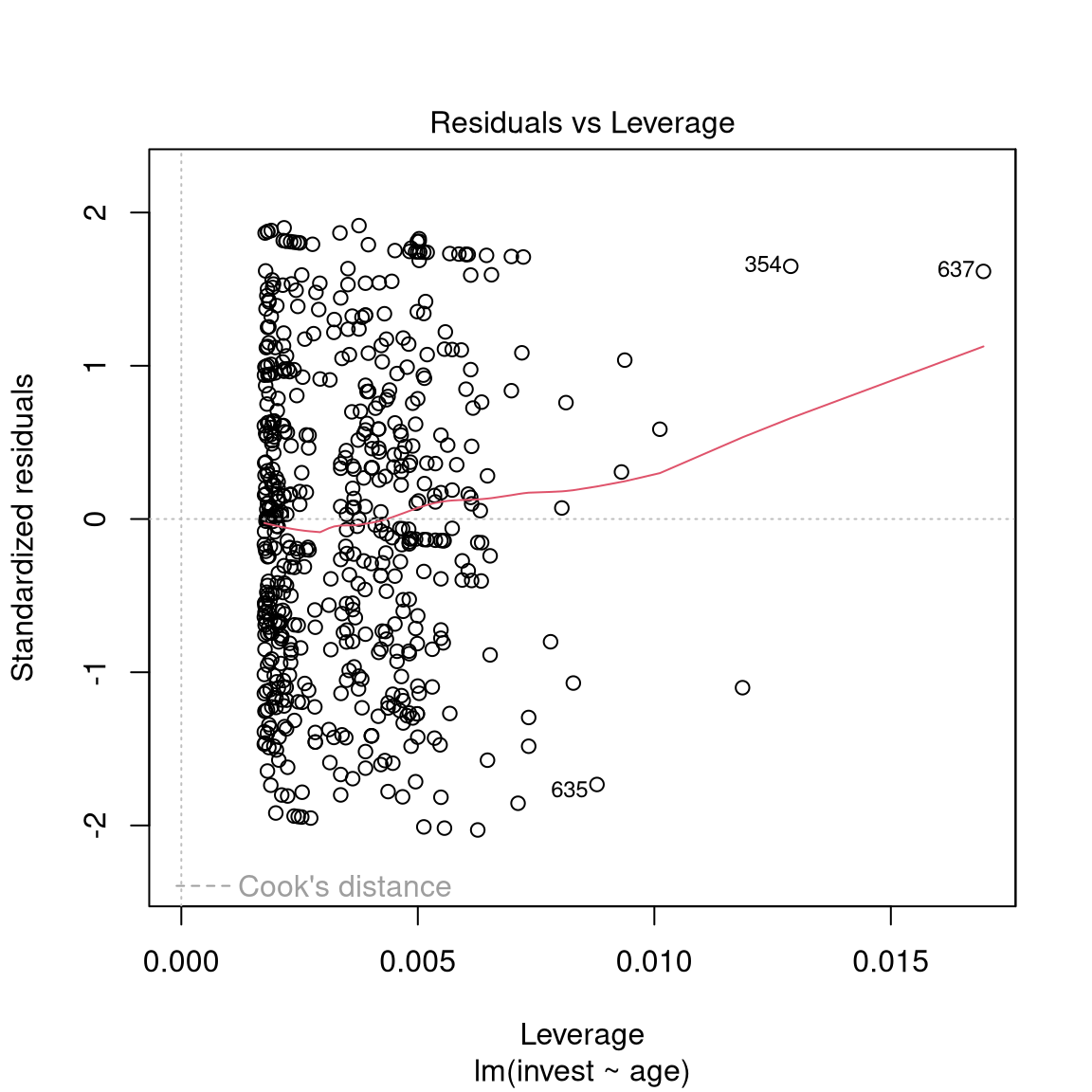
13.5.5 Diagnostic plots
Basic display: Residuals vs. fitted. Also some form of assessment of (non-)normality.

Further plotting options:
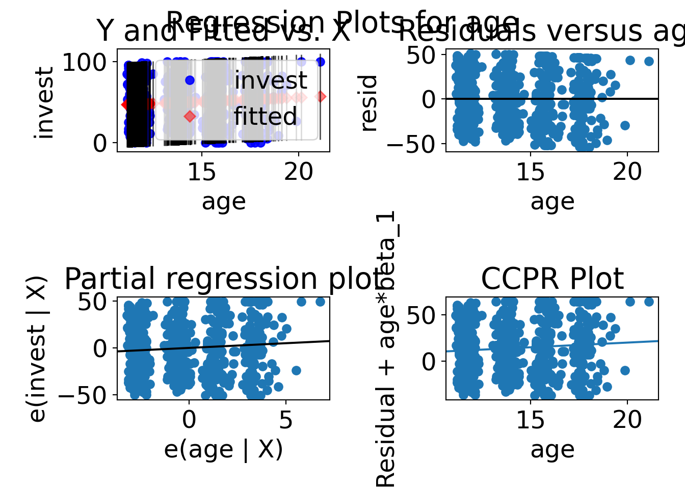
Python
statsmodels provides plots of regression results against one regressor.
The function plot_regress_exog() plots four graphs:
1. endog versus exog
2. residuals versus exog
3. fitted versus exog
4. fitted plus residual versus exog
The function diagnostic_plots() produces linear regression diagnostic plots similar to the R function plot(). It uses the library seaborn for statistical data visualization. Q-Q plot rather than histogram is used for assessing (non-)normality.
import seaborn as sns
from statsmodels.graphics.gofplots import ProbPlot

def diagnostic_plots(m):
    """
    Produces linear regression diagnostic plots like the function 'plot()' in R.

    :param m: Object of type statsmodels.regression.linear_model.OLSResults
    """
    # normalized residuals
    norm_residuals = m.get_influence().resid_studentized_internal
    # absolute squared normalized residuals
    residuals_abs_sqrt = np.sqrt(np.abs(norm_residuals))
    # leverage, from statsmodels internals
    leverage = m.get_influence().hat_matrix_diag

    #_, axes = plt.subplots(nrows=2, ncols=2)
    #plt.subplots_adjust(wspace=0.2, hspace=0.2)

    fig = plt.figure()
    # Residuals vs Fitted
    ax = fig.add_subplot(2, 2, 1)
    sns.residplot(x=m.fittedvalues.values, y=m.resid.values, ax=ax, lowess=True, line_kws={'color': "red"})
    ax.set(title="Residuals vs Fitted", xlabel="Fitted values", ylabel="Residuals");

    # Normal Q-Q plot
    ax = fig.add_subplot(2, 2, 2)
    QQ = ProbPlot(norm_residuals)
    QQ.qqplot(line='45', ax=ax)
    ax.set(title="Normal Q-Q", xlabel="Theoretical Quantiles", ylabel="Standardized Residuals")

    # Scale-Location
    ax = fig.add_subplot(2, 2, 3)
    sns.regplot(x=m.fittedvalues.values, y=residuals_abs_sqrt, ax=ax,
                lowess=True, line_kws={'color': 'red'});
    ax.set(title="Scale-Location", xlabel="Fitted values", ylabel="$\sqrt{|Standardized~Residuals|}$")

    # Residuals vs Leverage
    ax = fig.add_subplot(2, 2, 4)
    sns.regplot(x=leverage, y=norm_residuals, ax=ax, lowess=True,
                line_kws={"color": "red", "label": "Cook's distance"});
    ax.set_xlim(0, max(leverage)+0.001)
    ax.set(title="Residuals vs Leverage", xlabel="Leverage", ylabel="Standardized Residuals")
    ax.legend(loc="lower right")

    fig.subplots_adjust(wspace=.5, hspace=0.7)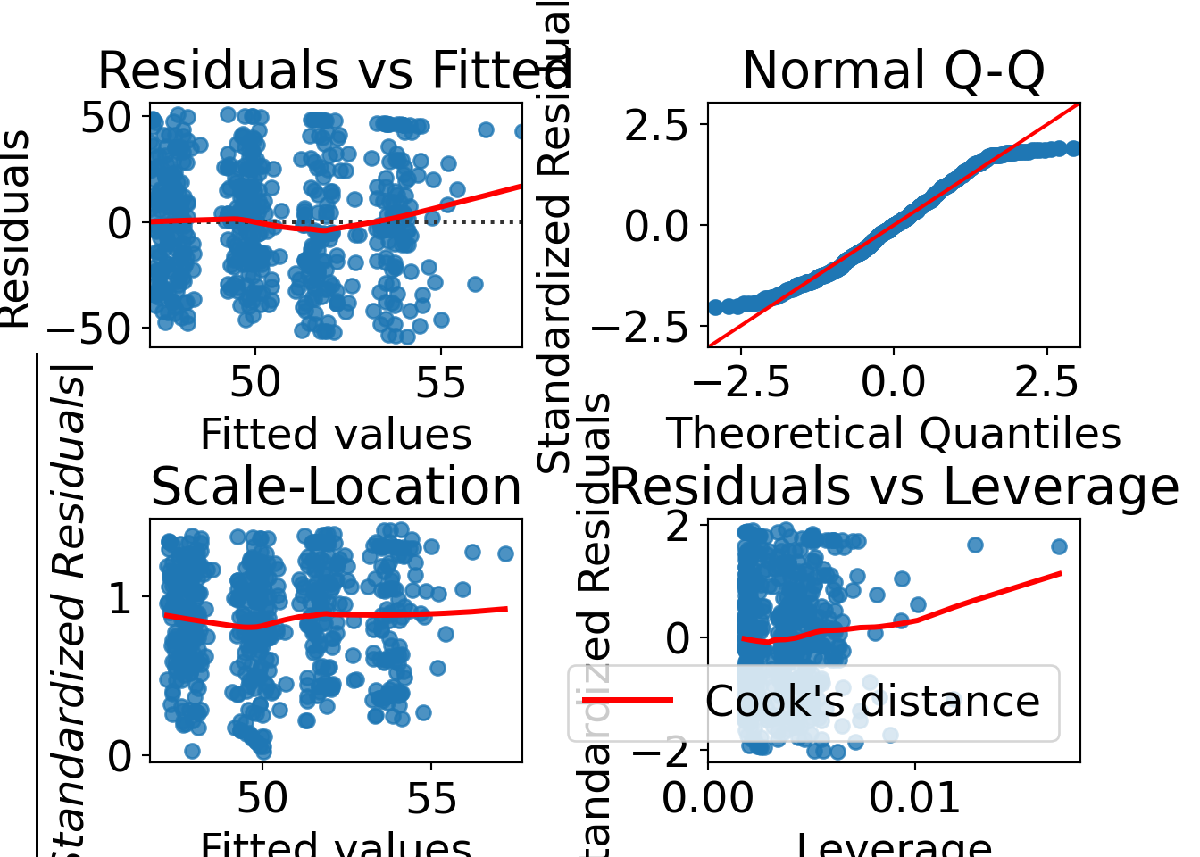
13.5.6 Extractor functions
R
| Function | Description |
|---|---|
print() |
Simple printed display |
summary() |
Standard regression output (including \(t\)-tests) |
anova() |
Comparison of nested models (including \(F\)-test) |
plot() |
Diagnostic plots |
predict() |
Predictions for new data \(\hat y_i = x_i^\top \hat \beta\) |
fitted() |
Extract fitted values for learning data \(\hat y_i = x_i^\top \hat \beta\) |
residuals() |
Extract residuals \(\hat \varepsilon_i = y_i - \hat y_i\) |
coef() |
Extract estimated coefficients \(\hat \beta\) |
vcov() |
Extract estimated variance-covariance matrix \(\hat \sigma^2 (X^\top X)^{-1}\) |
confint() |
Confidence intervals for coefficients \(\hat \beta \pm t_{n-k; 1 - \alpha/2} \cdot \widehat{\mathit{SD}(\hat \beta)}\) |
nobs() |
Number of observations \(n\) |
deviance() |
Residual sum of squares \(\sum_{i = 1}^n (y_i - \hat y_i)^2\) |
logLik() |
Log-likelihood (assuming Gaussian errors) |
AIC() |
Akaike information criterion (with default penalty \(2\)) |
BIC() |
Bayes information criterion (with penalty \(\log(n)\) |
model.matrix() |
Model matrix (or regressor matrix) \(X\) |
model.frame() |
Data frame with (possibly transformed) learning data |
formula() |
Regression formula y ~ x1 + x2 + ... |
terms() |
Symbolic representation of the terms in a regression model |
Python
| Class / Library | Method / Property | Description |
|---|---|---|
| built-in | print() |
Simple printed display |
| User defined | diagnostic_plots() |
R-style diagnostic plots |
linear_model.OLSResults |
summary() |
Standard regression output (including \(t\)-tests) |
linear_model.OLSResults |
anova_lm() |
Comparison of nested models (including \(F\)-test) |
linear_model.OLSResults |
predict() |
Predictions for new data \(\hat y_i = x_i^\top \hat \beta\) |
linear_model.OLSResults |
cov_params() |
Extract estimated variance-covariance matrix \(\hat \sigma^2 (X^\top X)^{-1}\) |
linear_model.OLSResults |
conf_int() |
Confidence intervals for coefficients \(\hat \beta \pm t_{n-k; 1 - \alpha/2} \cdot \widehat{\mathit{SD}(\hat \beta)}\) |
linear_model.OLSResults |
fittedvalues |
Extract fitted values for learning data \(\hat y_i = x_i^\top \hat \beta\) |
linear_model.OLSResults |
resid |
Extract residuals \(\hat \varepsilon_i = y_i - \hat y_i\) |
linear_model.OLSResults |
params |
Extract estimated coefficients \(\hat \beta\) |
linear_model.OLSResults |
nobs |
Number of observations \(n\) |
linear_model.OLSResults |
mse_resid |
Mean squared error of the residuals \(\frac{1}{n}\sum_{i = 1}^n (y_i - \hat y_i)^2\) |
linear_model.OLSResults |
llf |
Log-likelihood (assuming Gaussian errors) |
linear_model.OLSResults |
aic |
Akaike information criterion (with penalty \(2\)) |
linear_model.OLSResults |
bic |
Bayes information criterion (with penalty \(\log(n)\) |
linear_model.OLS |
data.frame |
Data frame with (possibly transformed) learning data |
linear_model.OLS |
formula |
Regression formula y ~ x1 + x2 + ... |
Some illustrations and examples:
Fitted values and residuals:
Coefficients/Parameters:
Variance-covariance matrix and standard deviations:
Regressor matrix and data frame with learning data: