Chapter 6 Principal component analysis
6.1 Motivation
Recall: Projections of the data matrix \(X\) from \(\mathbb{R}^p\) to \(\mathbb{R}^2\) are convenient for visualizations as shown in the pairwise scatter plots.
Problems:
- There is a large number of possible \(2\)-dimensional projections without particular order.
- Only projections along the axes are considered.
Solution: Consider a set of linear combinations \(X a_j\) \((j = 1, \dots, p)\) with coefficients \(a_j\) chosen such that \(X a_1\) is the “most interesting” linear combination, \(X a_2\) the “second most interesting” etc.
6.2 Algorithm
Statistically: Data analyses try to explain variation in empirical data.
Thus: “Interesting” typically means “captures a lot of variance”.
Geometrically: By constructing the linear combinations \(XA\) a new coordinate system is established where the first variable provides the “most information” about variations in the data. Subsequently, the second variable provides the “most information” of what is not yet explained by the first variable etc.
Hopefully: The first few of the new variables (e.g., \(q = 1\) or \(q = 2\), …) already capture most of the overall information/variance and the remaining \(p - q\) variables can be neglected in the subsequent analysis.
Jargon:
- The new variables constructed through linear combinations are called principal components.
- Principal component analysis (PCA) is often used for dimension reduction.
- Sometimes also called factor analysis.
- The coefficients \(a_j\) from the linear combinations are also known as loadings.
Construction: For the first principal component optimize \[ \max_{a} V(X a) ~=~ \max_{a} a^\top S a \] where \(S = V(X)\) is the covariance matrix of the data \(X\).
However: By increasing the coefficients \(a \rightarrow \infty\) the variance \(V(X a) \rightarrow \infty\) which is not useful.
Therefore: Make the problem identifiable by optimizing the variance under the constraint \[ a^\top a = 1. \]
Solution: Optimize the Lagrange function \[ f(a, \lambda) \quad = \quad a^\top S a \; - \; \lambda(a^\top a - 1) \]
First order conditions: Take derivative wrt. \(a\) and \(\lambda\) and set to \(0\).
\[\begin{eqnarray*} \frac{\partial f(a, \lambda)}{\partial a} & = & 0 \\ 2 S a \; - \; 2 \lambda a & = & 0 \\ S a & = & \lambda a \end{eqnarray*}\]
Jargon: A vector \(a\) with this property is known in linear algebra as eigenvector of the matrix \(S\) and \(\lambda\) is the corresponding eigenvalue.
Furthermore: The derivative wrt. \(\lambda\) yields the constraint
\[\begin{eqnarray*} \frac{\partial f(a, \lambda)}{\partial \lambda} & = & 0 \\ a^\top a & = & 1 \end{eqnarray*}\]
In linear algebra: Known as the eigendecomposition of a matrix \(S\) (here: the covariance matrix). This is a standard method, easily available in numerical software.
Alternatively: A closely-related method in linear algebra is the singular value decomposition which can also be used to carry out principal component analyses.
Therefore: The variance of the first principal component \(X a\) is given by the eigenvalue \(\lambda\).
\[\begin{eqnarray*} V(X a) & = & a^\top S a ~=~ a^\top \lambda a ~=~ \lambda a^\top a \\ & = & \lambda. \end{eqnarray*}\]
More generally: If there are no linear dependencies between the variables/columns in \(X\), the matrix \(S\) has \(p\)~eigenvalues \(\lambda_1, \dots, \lambda_p\) with corresponding eigenvectors \(a_1, \dots, a_p\).
Order: Sorting the eigenvalues so that \(\lambda_1 > \lambda_2 > \dots > \lambda_p\), yields the linear combinations \(X a_1\) with highest variance, \(X a_2\) with the second-highest variance, etc.
Problem: If the variables/columns in \(X\) have very different scales, the principal components will be dominated by those variables with high variance.
Solution: Standardize all variables to have the same scale with variance \(1\). This gives every variable exactly the same prior weight or importance.
Standardization: Scale matrix \(X\) to \(\hat X\) so that each column as mean \(0\) and variance \(1\).
\[ \hat x_{ij} \quad = \quad \frac{x_{ij} - \overline x_j}{\sigma_j} \]
Technically: This corresponds to computing the eigendecomposition of the correlation matrix rather than the covariance matrix.
6.3 Standardization: Mean/variance
Example:
Original data (selection of observations/variables):
##                  SA01.tennis SA05.swim SA17.shop SA21.museum
## Austria (Vienna)       0.038     0.414     0.086       0.057
## Spain                  0.004     0.101     0.227       0.405
Means and standard deviations (across all observations):
##                  SA01.tennis SA05.swim SA17.shop SA21.museum
## mean                   0.021     0.312     0.185       0.143
## sd                     0.012     0.104     0.057       0.104
Data scaled to mean \(0\) and variance \(1\):
##                  SA01.tennis SA05.swim SA17.shop SA21.museum
## Austria (Vienna)       1.419     0.986    -1.742      -0.824
## Spain                 -1.385    -2.021     0.731       2.512
6.4 Illustration
Example: PCA for GSA data, aggregated by country (\(n = 15\) countries and \(p = 8\) activities) and mean/variance scaling.
- PCA obtains the \(8 \times 8\) rotation matrix \(A\) with the coefficients/eigenvectors \(a_1, \dots, a_8\).
- The corresponding eigenvalues \(\lambda_1, \dots, \lambda_8\) indicate the variance “explained” by the corresponding principal component.
- To select the number of required principal components consider the fraction of variance explained of the total variance (here: \(8\) due to scaling), i.e., \(\lambda_k/(\sum_{j=1}^8\lambda_j)=\lambda_k/8\).
- Principal components are defined only up to the sign which may differ across implementations.
Eigenvectors: Rotation matrix \(A\).
| Activity | \(PC_1\) | \(PC_2\) | \(\dots\) |
|---|---|---|---|
| Tennis | \(-0.351\) | \(-0.287\) | |
| Cycling | \(-0.387\) | \(-0.202\) | |
| Riding | \(-0.315\) | \(-0.477\) | |
| Swimming | \(-0.363\) | \(0.249\) | |
| Shopping | \(0.344\) | \(0.387\) | |
| Concerts | \(0.351\) | \(-0.303\) | |
| Sightseeing | \(0.384\) | \(-0.232\) | |
| Museum | \(0.327\) | \(-0.541\) |
Illustration: Computation of the principal components for selected observations in the scaled GSA data.
##                  SA01.tennis SA02.cycle SA03.ride SA05.swim SA17.shop SA18.concert
## Austria (Vienna)       1.419      1.399     1.599     0.986    -1.742       -1.121
## Spain                 -1.385     -1.490    -1.035    -2.021     0.731        1.223
##                  SA19.sight SA21.museum
## Austria (Vienna)     -1.350      -0.824
## Spain                 2.463       2.512
\(\mathit{PC}_1\) for Austria (Vienna): \(-3.682 =\)
\(-0.351 \cdot 1.419-0.387 \cdot 1.399-0.315 \cdot 1.599\) \(-0.363 \cdot 0.986+0.344 \cdot (-1.742)+0.351 \cdot (-1.121)\) \(+0.384 \cdot (-1.350)+0.327 \cdot (-0.824)\).
\(\mathit{PC}_1\) for Spain: \(4.570 =\)
\(-0.351 \cdot (-1.385)-0.387 \cdot (-1.490)-0.315 \cdot (-1.035)\) \(-0.363 \cdot (-2.021)+0.344 \cdot 0.731+0.351 \cdot 1.223\) \(+0.384 \cdot 2.463+0.327 \cdot 2.512\).
\(\mathit{PC}_2\) for Austria (Vienna): \(-0.783 =\)
\(-0.287 \cdot 1.419-0.202 \cdot 1.399-0.477 \cdot 1.599\) \(+0.249 \cdot 0.986+0.387 \cdot (-1.742)-0.303 \cdot (-1.121)\) \(-0.232 \cdot (-1.350)-0.541 \cdot (-0.824)\).
\(\mathit{PC}_2\) for Spain: \(-1.327 =\)
\(-0.287 \cdot (-1.385)-0.202 \cdot (-1.490)-0.477 \cdot (-1.035)\) \(+0.249 \cdot (-2.021)+0.387 \cdot 0.731-0.303 \cdot 1.223\) \(-0.232 \cdot 2.463-0.541 \cdot 2.512\).
Interpretation: Consider signs and absolute values of the coefficients.
- All \(\mathit{PC}_1\) coefficients have a similar absolute value but differing signs.
- Thus, \(\mathit{PC}_1\) contrasts variables with negative coefficients (sports activities: tennis, cycling, riding, swimming) and those with positive coefficients (cultural activities: shopping, concerts, sightseeing, museum).
- A high positive value for \(\mathit{PC}_1\) for a given country indicates high interest in cultural activities and low interest in sports activities.
- \(\mathit{PC}_2\) contrasts shopping/swimming with the remaining activities.
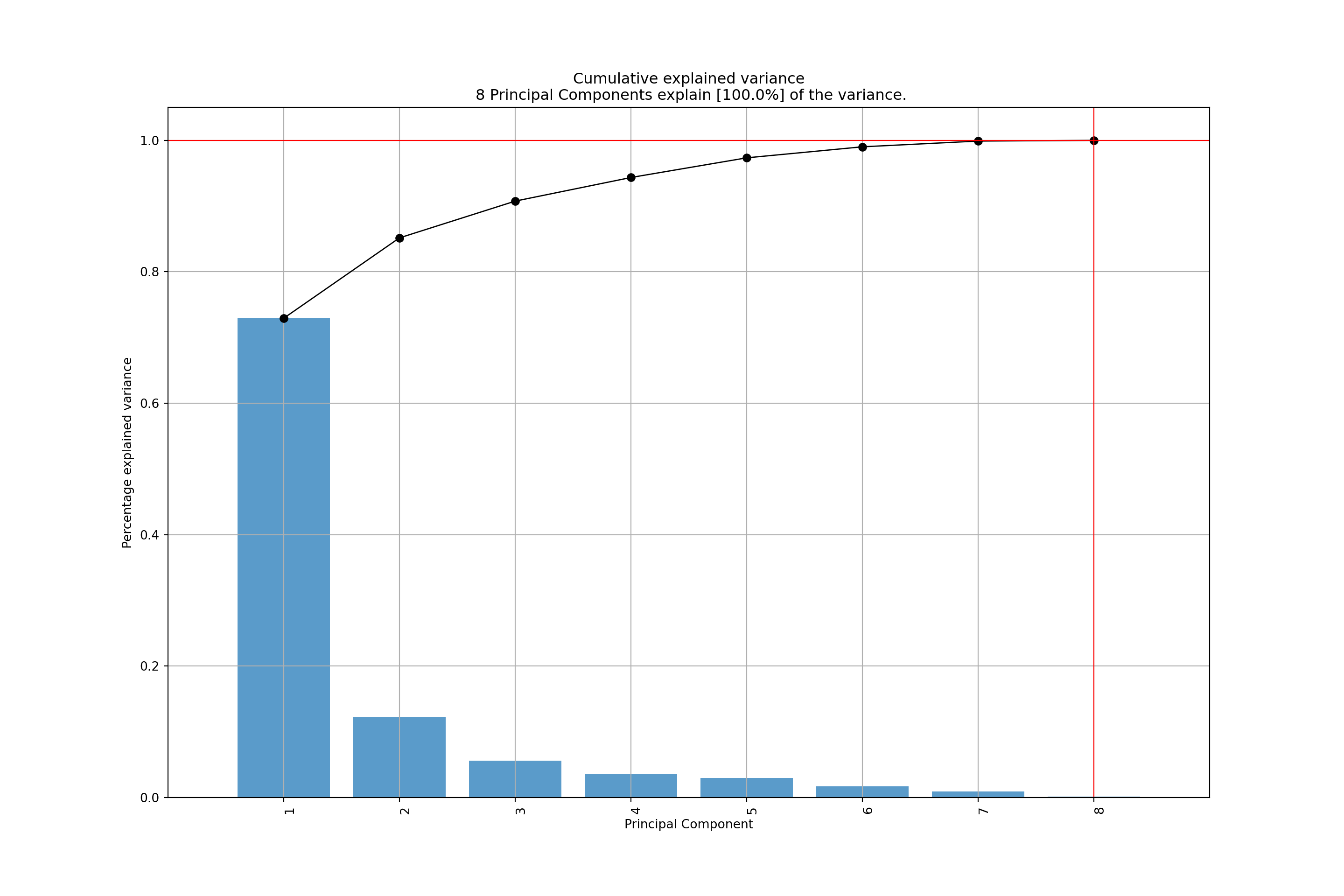
Variance explained:
- \(\mathit{PC}_1\) captures 73% of the total variance.
- \(\mathit{PC}_2\) captures only 12%.
- Visualization by bar plot is known as scree plot.
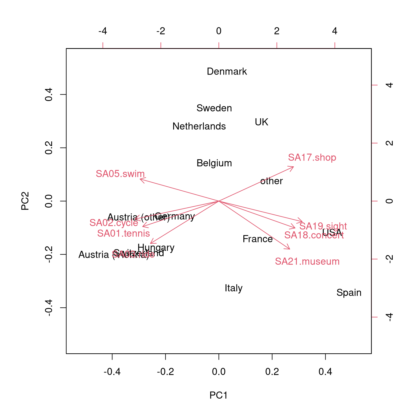
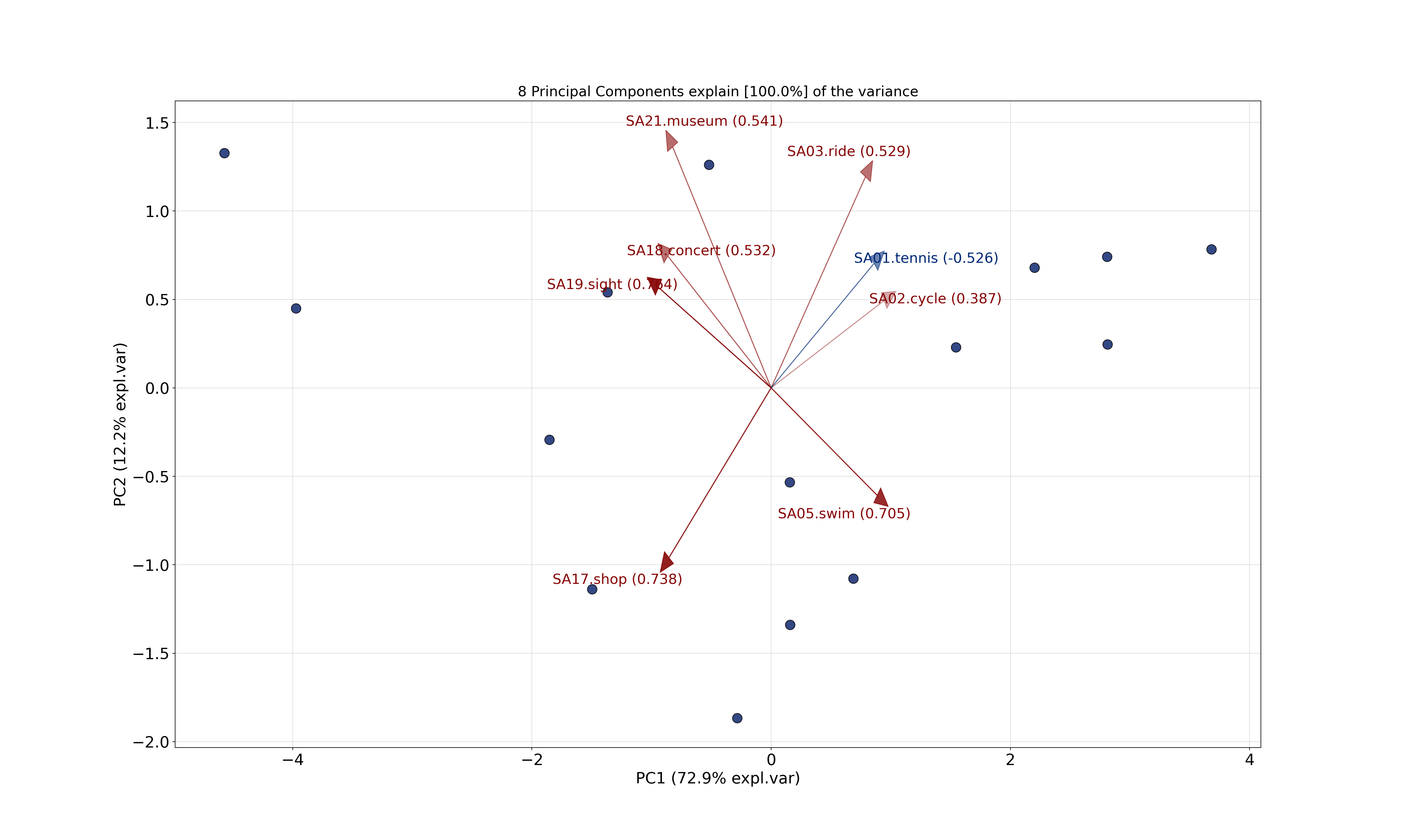
Further visualization:
- Pairwise scatter plots for the first few principal components.
- Known as biplots when combined with projection of the original axes.
- Axes with similar directions (i.e., separated by small angles only) capture similar concepts.
- More precisely, angles between the axes correspond to correlations (or covariances) between the underlying variables.

6.5 Tutorial
As in previous chapters, the Guest Survey Austria data are used for illustration, considering the interest in \(p = 8\) summer activities aggregated within \(n = 15\) countries. See Chapter 3 for the data preprocessing, or download the data set directly: gsa-country.csv, gsa-country.rda.
6.5.1 Setup
Python
Install the pca library https://pypi.org/project/pca/. You can use the command pip install pca
# Make sure that the required libraries are installed.
# Import the necessary libraries and classes:
import pandas as pd
import numpy as np
from matplotlib import pyplot as plt
import seaborn as sns

from pca import pca

pd.set_option("display.precision", 4) # Set display precision to 4 digits in pandas and numpy.
# Load dataset
gsa = pd.read_csv("gsa-country.csv", index_col=0, header=0)
# Normalize
gsa = (gsa - gsa.mean()) / gsa.std()Note: We have normalized the data here instead of using the normalize attribute of pca. The reason is that R and pandas use an unbiased estimator to compute the std while pca uses a biased estimator that gives different results.
6.5.2 Analysis
R
In base R, basic principal component analysis (PCA) can be carried out using the prcomp() function. This comes with both a formula interface and a
default interface based on a matrix or data frame which can optionally be scaled
(setting scale = TRUE). For the resulting object a number of useful methods
are available:
print(): Standard deviations and rotation coefficients.summary(): Individual and cumulative proportion of variance.plot(): Scree plot of variances.biplot(): Biplot of the first two principal components.predict(): Predict principal components for learning data or new data.
Extended PCA functionality is available in a number of packages such as the
principal() function in the psych package. Here, using the base prcomp()
suffices though.
For the Guest Survey Austria we employ the scaled PCA (i.e., based on correlations rather than covariances) to account for the very different scales of the eight variables:
## Standard deviations (1, .., p=8):
## [1] 2.4154816 0.9890608 0.6690866 0.5361590 0.4893967 0.3662942 0.2645973 0.0914957
##
## Rotation (n x k) = (8 x 8):
##                    PC1       PC2        PC3       PC4        PC5        PC6        PC7
## SA01.tennis  -0.351051 -0.287018 -0.4175851  0.526335  0.3002696  0.2544644 -0.4190326
## SA02.cycle   -0.386754 -0.202268 -0.0374428  0.325919 -0.0155493 -0.3809876  0.7193745
## SA03.ride    -0.315178 -0.476968  0.3495266 -0.528725  0.5020926  0.1329511  0.0270175
## SA05.swim    -0.362934  0.248650  0.4051869  0.172497 -0.2900876  0.7046026  0.1754956
## SA17.shop     0.344053  0.386707  0.0945613  0.260554  0.7376597  0.1558362  0.2912806
## SA18.concert  0.351151 -0.303023 -0.5316426 -0.237602 -0.1100615  0.4985035  0.4063317
## SA19.sight    0.384426 -0.231945  0.3837163  0.200675 -0.0689462 -0.0170732 -0.1496854
## SA21.museum   0.326593 -0.540572  0.3147245  0.377928 -0.1110837  0.0536039  0.0550255
##                     PC8
## SA01.tennis   0.1116938
## SA02.cycle    0.1974618
## SA03.ride     0.0306950
## SA05.swim     0.0332537
## SA17.shop    -0.0445369
## SA18.concert  0.1415848
## SA19.sight    0.7638447
## SA21.museum  -0.5839493
Python
Carry out basic principal component analysis (PCA) in {python} using the pca library.
# Initialize to reduce the data up to the number of components that explain 95% of the variance.
#gsa_pca = pca(n_components=0.95) # Automatically determine the number of components to explain 95% of variance

gsa_pca = pca(n_components=8, normalize=False)

# Fit transform
pca_results = gsa_pca.fit_transform(gsa)
## [pca] >Extracting column labels from dataframe.
## [pca] >Extracting row labels from dataframe.
## [pca] >The PCA reduction is performed on the [8] columns of the input dataframe.
## [pca] >Fit using PCA.
## [pca] >Compute loadings and PCs.
## [pca] >Compute explained variance.
## [pca] >Outlier detection using Hotelling T2 test with alpha=[0.05] and n_components=[8]
## [pca] >Multiple test correction applied for Hotelling T2 test: [fdr_bh]
## [pca] >Outlier detection using SPE/DmodX with n_std=[3]## PC1 PC2 PC3 PC4 PC5 PC6 PC7 PC8
## SA01.tennis 0.3511 0.2870 0.4176 -0.5263 0.3003 0.2545 -0.4190 0.1117
## SA02.cycle 0.3868 0.2023 0.0374 -0.3259 -0.0155 -0.3810 0.7194 0.1975
## SA03.ride 0.3152 0.4770 -0.3495 0.5287 0.5021 0.1330 0.0270 0.0307
## SA05.swim 0.3629 -0.2487 -0.4052 -0.1725 -0.2901 0.7046 0.1755 0.0333
## SA17.shop -0.3441 -0.3867 -0.0946 -0.2606 0.7377 0.1558 0.2913 -0.0445
## SA18.concert -0.3512 0.3030 0.5316 0.2376 -0.1101 0.4985 0.4063 0.1416
## SA19.sight -0.3844 0.2319 -0.3837 -0.2007 -0.0689 -0.0171 -0.1497 0.7638
## SA21.museum -0.3266 0.5406 -0.3147 -0.3779 -0.1111 0.0536 0.0550 -0.5839The output reports the standard deviations of all components (square root of the eigenvalues) along with the corresponding rotations (eigenvectors). Here, the first component is the only one to have a higher variance than each of the original scaled variables (all of which by definition have a unit variance). This component contrasts interest in sports activities with interest in cultural activities. The second component already accounts for a substantially lower variance and contrasts swimming and shopping with the remaining activities.
The variance accounted for is reported in more detail by:
R
## Importance of components:
##                          PC1   PC2   PC3    PC4    PC5    PC6     PC7     PC8
## Standard deviation     2.415 0.989 0.669 0.5362 0.4894 0.3663 0.26460 0.09150
## Proportion of Variance 0.729 0.122 0.056 0.0359 0.0299 0.0168 0.00875 0.00105
## Cumulative Proportion 0.729 0.852 0.908 0.9435 0.9734 0.9902 0.99895 1.00000This shows that almost three quarters of the overall variance is already captured by the first principal component alone. Visually the same is brought out by the scree plot:

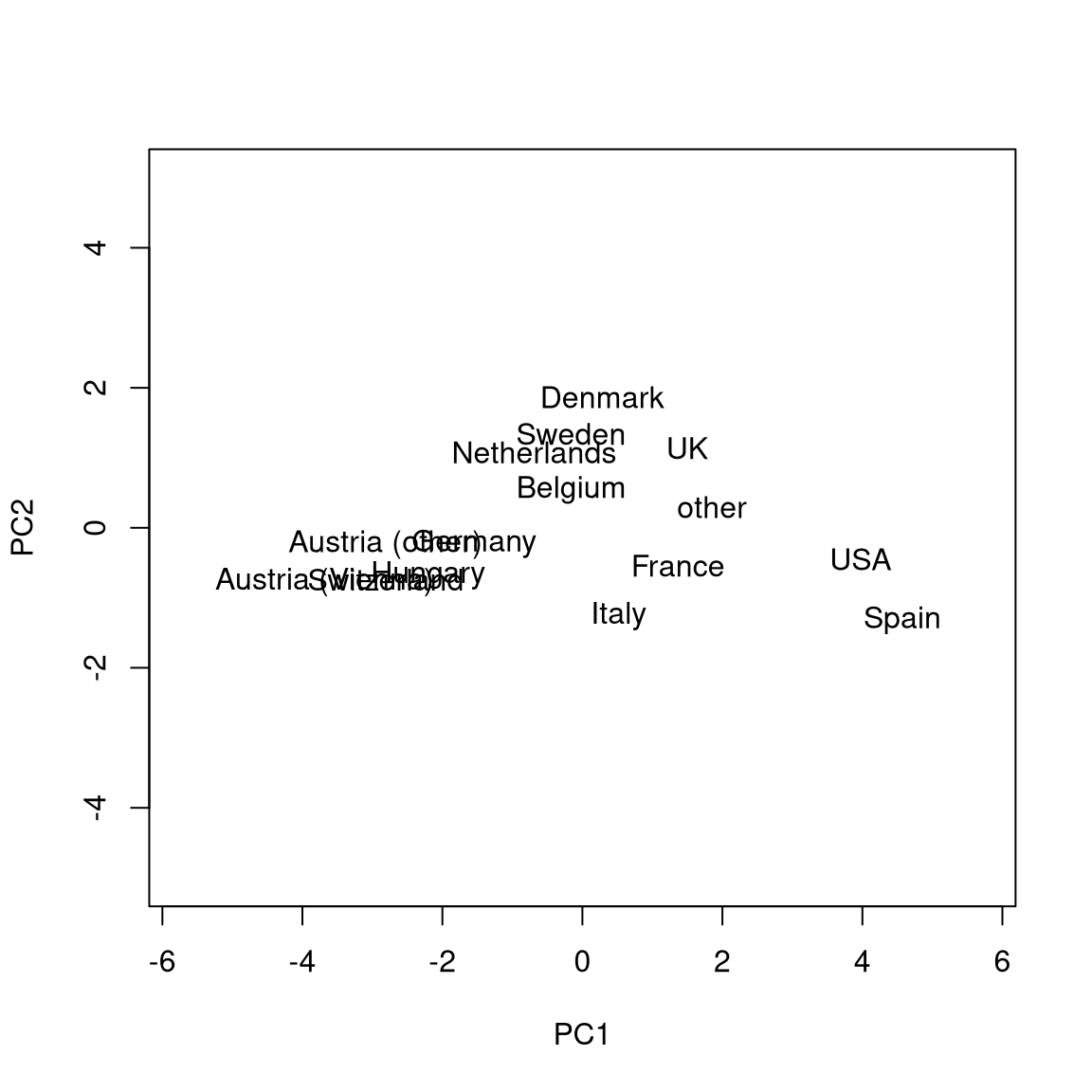
Therefore, when interpreting the biplot more attention should be given to the first principal component (x-axis) rather than the second principal component (y-axis).
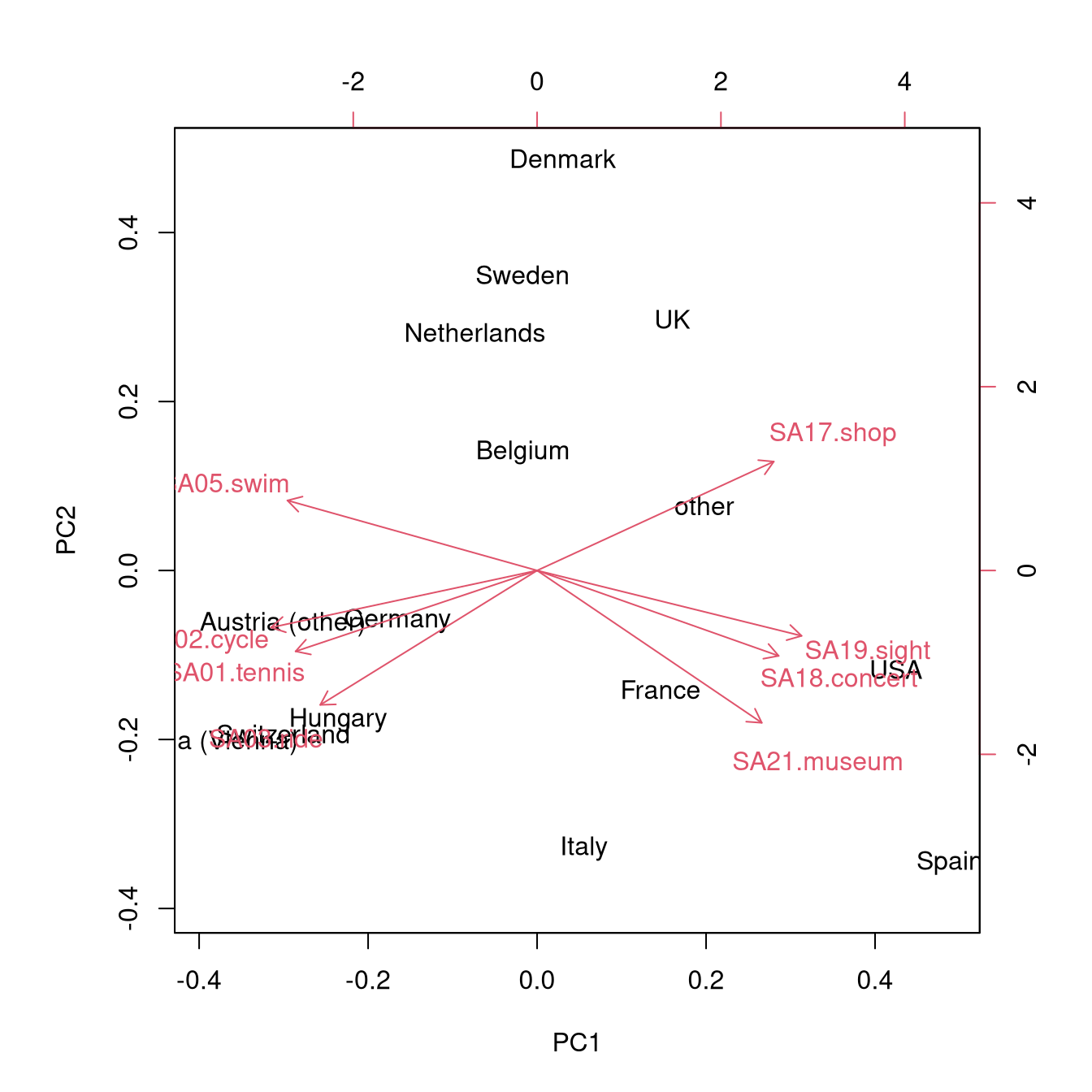
The contrast between countries with interest mainly in sports activities (Austria, Switzerland, Hungary, Germany), mainly in cultural activities (Spain, USA) is brought out nicely, with the other countries being somewhere in between.
6.5.3 Computational details
Here, we show how to replicate various of the involved computations “by hand”,
beginning with the variances and corresponding (cumulative) proportions from the
summary() in R or pca_results in Python:
R
## [1] 5.83455156 0.97824124 0.44767693 0.28746649 0.23950914 0.13417147 0.07001171
## [8] 0.00837146## [1] 0.72931895 0.12228016 0.05595962 0.03593331 0.02993864 0.01677143 0.00875146
## [8] 0.00104643## [1] 0.729319 0.851599 0.907559 0.943492 0.973431 0.990202 0.998954 1.000000Python
## PC1    5.8346
## PC2    0.9782
## PC3    0.4477
## PC4    0.2875
## PC5    0.2395
## PC6    0.1342
## PC7    0.0700
## PC8    0.0084
## dtype: float64## PC1 0.7293
## PC2 0.1223
## PC3 0.0560
## PC4 0.0359
## PC5 0.0299
## PC6 0.0168
## PC7 0.0088
## PC8 0.0010
## dtype: float64## PC1 0.7293
## PC2 0.8516
## PC3 0.9076
## PC4 0.9435
## PC5 0.9734
## PC6 0.9902
## PC7 0.9990
## PC8 1.0000
## dtype: float64The principal components itself can be extracted (or predicted) for both the original learning data or a new data set with:
R
##                        PC1       PC2
## Austria (Vienna) -3.682230 -0.782833
## Austria (other)  -2.813329 -0.245321
## Belgium          -0.156518  0.534210
## Denmark           0.282693  1.867547
This can be replicated by first scaling the original gsa data to zero mean and
variance 1 with scale() and then using a matrix multiplication %*% with the
rotation coefficients:
##                        PC1       PC2
## Austria (Vienna) -3.682230 -0.782833
## Austria (other)  -2.813329 -0.245321
## Belgium          -0.156518  0.534210
## Denmark 0.282693 1.867547Finally, we can create a scatter plot of the first two principal components with:
R
plot(gsa.pred[, 1:2], type = "n", xlab = "PC1", ylab = "PC2",
  xlim = c(-4.5, 4.5), ylim = c(-4.5, 4.5))
text(gsa.pred[, 1:2], rownames(gsa))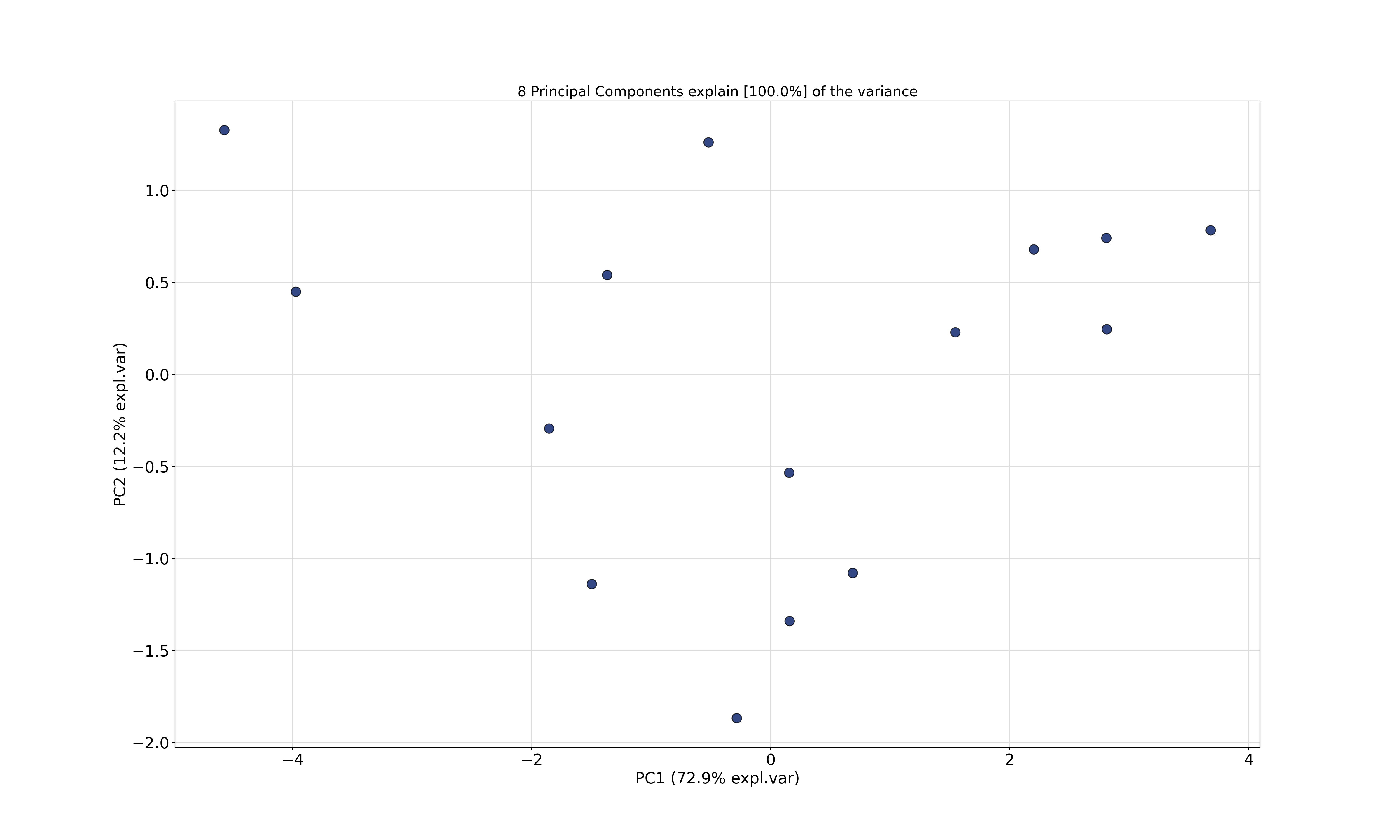
This first creates the plot without actually drawing any points (due to type ="n"). The x-axis and y-axis have the same scaling (xlim and ylim) to convey variance differences between the two components. Then, text() adds the row names of the data at the coordinates for the first two components.

6.5.4 Scaling
R
Above the scale() function was used to scale all columns of a data matrix to zero
mean and unit variance. In fact, the scale() function could also take a custom
center and scale argument for different standardizations. Moreover, it
returns the centers/scales employed as an attribute to the scaled matrix. For
illustration we scale only the first five observations from the Guest Survey
Austria data:
##                  SA01.tennis SA02.cycle  SA03.ride SA05.swim  SA17.shop SA18.concert
## Austria (Vienna)    0.994283   0.980059  1.5484051  0.991017 -1.1052726    -0.852927
## Austria (other)     1.153242   1.173537  0.0473079  0.616826 -0.6898774    -0.521389
## Belgium            -1.025634  -0.454363  0.1524157 -0.483163  0.3658135     0.183807
## Denmark            -0.551207  -0.771671 -1.0305827  0.378806  1.4720059    -0.467343
## France             -0.570684  -0.927563 -0.7175460 -1.503486 -0.0426694     1.657852
##                  SA19.sight SA21.museum
## Austria (Vienna)  -1.216935   -0.756968
## Austria (other)   -0.767938   -0.534286
## Belgium            0.113978   -0.140912
## Denmark            0.647154   -0.307667
## France             1.223741    1.739834
## attr(,"scaled:center")
##  SA01.tennis   SA02.cycle    SA03.ride    SA05.swim    SA17.shop SA18.concert
##   0.02588724   0.12775917   0.00520096   0.34950762   0.15923770   0.03972197
##   SA19.sight  SA21.museum
##   0.29242791   0.09321951
## attr(,"scaled:scale")
##  SA01.tennis   SA02.cycle    SA03.ride    SA05.swim    SA17.shop SA18.concert
##   0.01214313   0.06109466   0.00504662   0.06539653   0.06654865   0.02749707
##   SA19.sight  SA21.museum
##   0.10571930   0.04720907
In this application, the "scaled:center" attribute can be interpreted as the
average interest in a summer activity (across the five countries considered
here). The "scaled:scale" attribute is the corresponding standard deviation.
For example, the average interest in tennis is rather low with moderate standard
deviation. In contrast, the average interest in swimming is much higher also at
a moderate standard deviation.
While the scale() function can be used to scale the data prior to calling prcomp(),
it is usually preferable to let prcomp() do the scaling. Thus, simply calling
prcomp(x, scale = TRUE) is better than prcomp(scale(x)) (which defaults to scale = FALSE).
The reason is that only in the former case prcomp() knows how exactly the data
were scaled and can store this information in the returned object.
Python
The input parameter normalize is used to scale all columns of the data matrix to zero mean and unit variance. However, we found out that pca uses a biased estimator to compute the standard deviation while R and pandas use an unbiased estimator that gives different results.
Therefore, we recommend to scale the data by hand before performing the pca.