Chapter 18 Reporting
In this chapter we will jump into ‘reporting’ using the R packages rmarkdown and knitr. This allows us to easily create (interactive) documents in different formats, such as HTML (like this document), PDF, or even Microsoft Word.
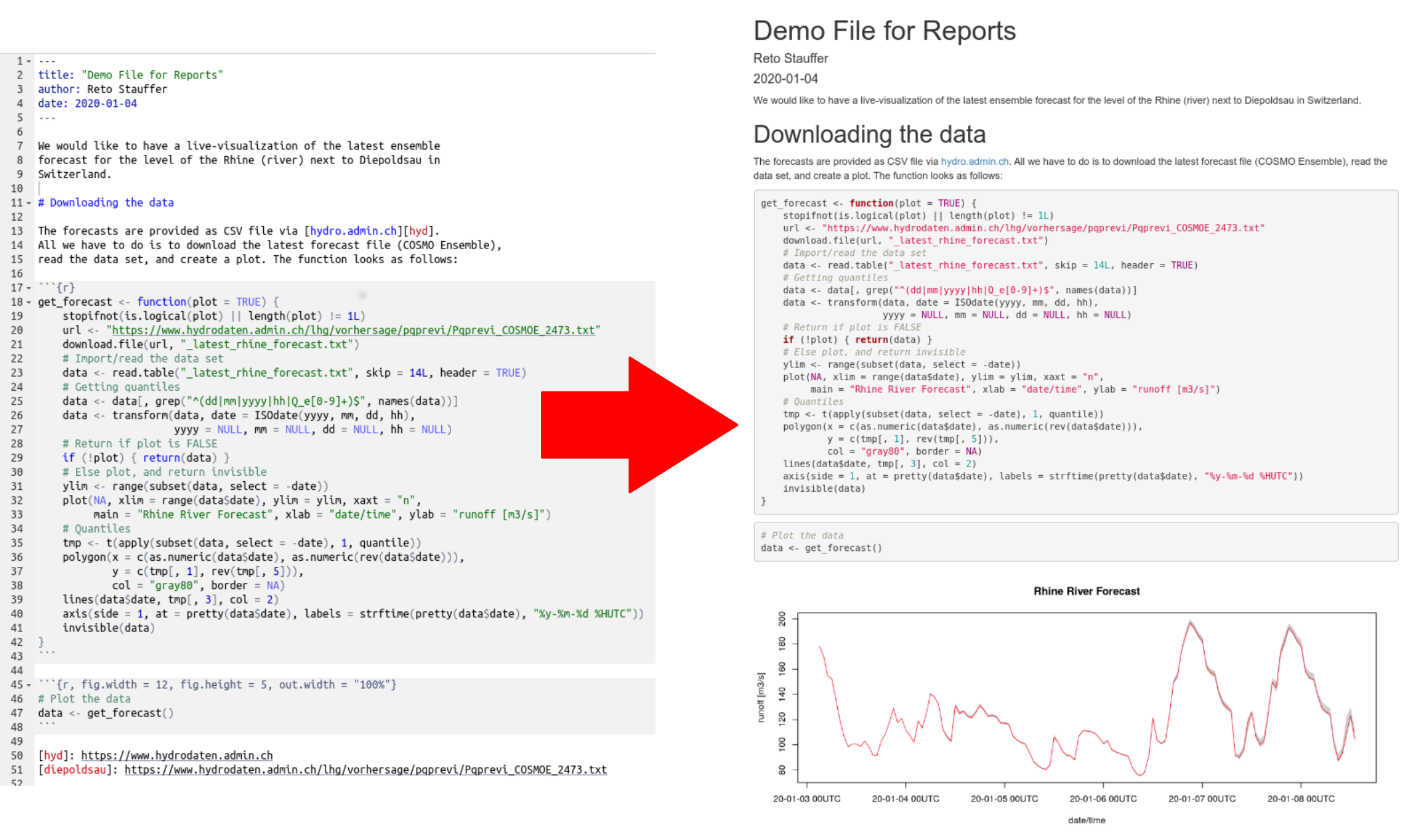
To increase the motivation: what we want to do is to bridge the
gap between pure code (source code; .R scripts) and a readable
file. This file can be for yourself, your colleague, sister, mum, or
boss. It helps to structure and document code and possible solutions.
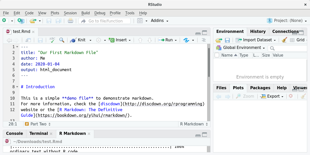
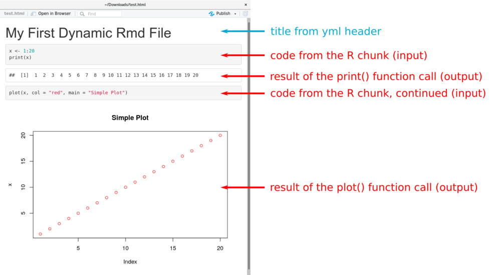
As an illustrative example (Rhine river runoff forecasts): we would
like to convert our code (left) into a nice html document (right):
18.1 Getting Started
As the title already indicates, R Markdown combines R and markdown. Markdown is a simple but powerful markup language. In contrast to programming languages, markup languages are used to structure text. Some well known markup languages are:
- markdown (which we will use here)
- HTML (HyperText Markup Language)
- Tex/LaTeX
Markup languages have specific elements which do not count as text (content) of the document, but allow to e.g., specify some text as title, make text bold face or italic, or set up enumerated lists. One example: if we want to define a section title we use:
#in markdown,<h1>...</h1>in HTML,- or
\section{...}in LaTeX.
Create New Document
While R scripts have the file ending .R, R markdown files have the
ending .Rmd (for R Markdown). RStudio supports you creating these
files. Let us create our first R Markdown file:
- Open your RStudio
- Create a new document by navigating through:
Files>New File>R Markdown. - A new window opens where you can select which type of document you want to create (Document, Presentation, Shiny, From Template). Select Document. You can also specify the title of the document and in which format it should be rendered. Leave this as it is for now.
- Press OK and you should end up with a new document (see below).
- Next step: save this new document (
File>Save; or press the save icon). Save the file astest.Rmd(important is the file ending) on your harddisc as if you would save an.Rscript.
The first things we have to know
You should now see something very similar to the screenshot below. By default,
RStudio creates an .Rmd document with some “demo-content”. Let us concentrate
on the first few lines of the document. This differs from what we have learned
from R scripts - --- or title: "Untitled" are no R commands and would
result in an error.
Important: this is no R code. That’s the header (to be precise, a so called
yml header). It defines the title of the document and how it should be rendered. In this
case we would like to have an html_document at the end.
Knit! When writing an R script we have a “source” button to run the script. Here we now have a button called “Knit”. Knit takes our R markdown file and converts it, in this case it tries to create an html document (via the R package knitr; thus “Knit”).

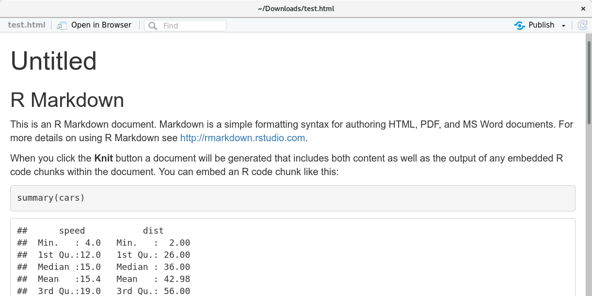
Try it. As RStudio gives us some demo content, we could try what’s happening if we knit it. Thus, press the “Knit” button. You will see some output in RStudio which comes from the knitr package. If everything works fine, RStudio opens the final html document and you should see this:
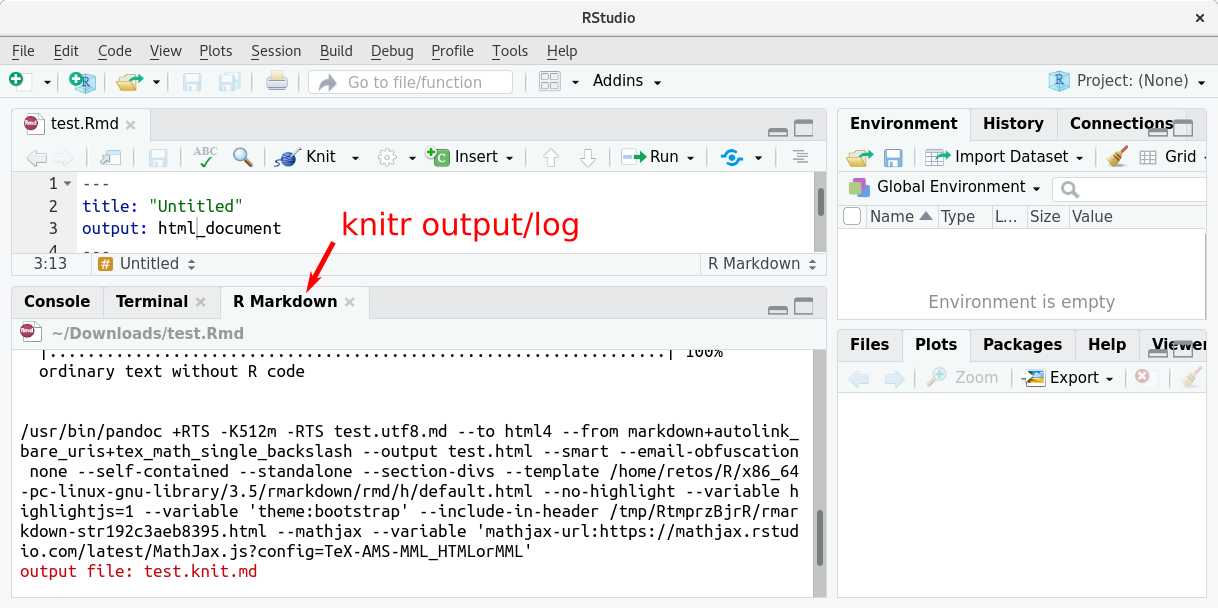
Fails? Well, it should not fail. However, if it does, there is an extra “R Markdown” output tab (bottom of your RStudio window). If errors occur, you should see the output down there.
The Output
In the example above we defined that we want to have an HTML file at the end
(output: html_document). After knitting the document RStudio will automatically
open the document. In addition, the HTML file is stored on your harddisc.
By default, an HTML file with the same name as your .Rmd file is stored in
the same folder as your .Rmd file. In the example above:
- Our
.Rmdfile is calledtest.Rmd. - In the same folder, you will now have a file
test.html.
Markdown Syntax
Before we start mixing markdown and R, let’s introduce the markdown syntax. There is only a handfull of commands we need to know - depending on the software you use this list might be extended (special commands for special applications).
<!DOCTYPE html PUBLIC “-//W3C//DTD HTML 4.0 Transitional//EN” “http://www.w3.org/TR/REC-html40/loose.dtd”>| Element | Markdown Syntax |
|---|---|
| Heading |
# Heading 1## Heading 2### Heading 3
|
| Bold |
**bold text**
|
| Italic |
_italic text_
|
| Strike trough |
~~strike trough~~
|
| Blockquote |
> blockquote
|
| Ordered List |
1. First item2. Second item3. Third item
|
| Unordered List |
- First item- Second item- Third item
|
| Code |
`code`
|
| Horizontal rules |
---
|
| Links |
[title](http://discdown.org)
|
| Images |

|
| Fenced Code Blocks |
```pow_fun <- function(x, y) { return(x**y)}```
|
| Math Expressions |
$x^2 = y^2 + z^2$
|
18.2 First Pure Markdown File
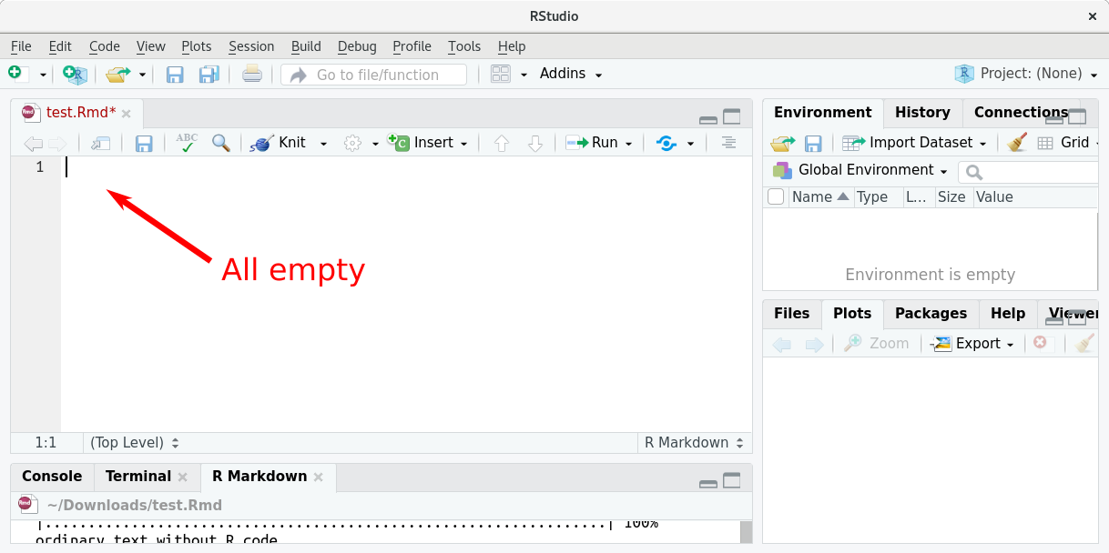
If you followed the guide above, you should have a file test.Rmd opened
in your Rstudio. Let us adjust the .Rmd file and delete everything
(in the code editor: simply mark everything and delete it) such that you
end up with an empty document (see below).
We will now create new content for this document (pure markdown).
- Define new yml header with title, author, date, and output format.
- Below the yml header, add some content. What we want to have is a section “Introduction” and “Results” with some text content. Not very meaningful - but we will extend this further in a minute.
Write/copy the following lines of code into your test.Rmd file:
---
title: "Our First Markdown File"
author: Me
date: 2020-01-04
output: html_document
---

# Introduction

This is a simple **demo file** to demonstrate markdown.
For more information, check the [discdown](http://discdown.org/rprogramming)
website or the [R Markdown: The Definitive Guide](https://bookdown.org/yihui/rmarkdown/).

# Results

## Part One

The file should be:

* Rendered.
* An HTML file should be created.
* Rstudio automatically openes the HTML file if successfully knit.

## Part Two

Not a lot to say, but we could try _italic text_, **bold text**,
and ~~strike trough~~ text. In addition, we can define `inline code`
elements (e.g., `p <- x**y`).
… such that you end up with this:
We can now render (knit) this file by pressing the “Knit” button again. If everything works well, a new window will pop up which looks as follows:
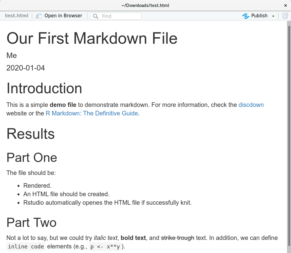
Great! First (R) markdown file rendered as HTML document. What have we done?
- Header: we defined a document title, author, and date.
- The content:
- The first section (“Introduction”; heading 1 denoted by
#) contains some text and two links (to discdown and the definitive R markdown guide). - The second section (“Results”;
#) itself has two subsections (heading 2, denoted by##) which contain an unordered list, and some text with text styling (bold face, italic, strike trough, and code).
- The first section (“Introduction”; heading 1 denoted by
So far, this has nothing to do with R markdown except that it is rendered via R and rmarkdown/knitr. But we could also do this without R (e.g., solely using pandoc). Let’s dive a bit deeper and combine Markdown with R.
18.3 First R Markdown File
To create ‘dynamic’ documents we can combine pure Markdown with R chunks. A chunk is nothing else than a block of R code. R chunks are “parts of R scripts” and have to contain executeable R code and/or comments.
This allows us to execute R commands on the fly. Whenever the document is rendered (‘knitted’) the R commands (scripts) will be executed and embedded in the final document.
When to use?
R markdown is very handy for different tasks. This online learning resource (discdown.org) is completely written in R markdown. If you took the course “Introduction to Programming: Programming in R” at the Universität Innsbruck, everything - from the PDF slides to the exercises, and even the quizzes - is/was based on R markdown.
For yourself
Rather than solely writing an R script, you may write a small R markdown file for yourself. Instead of having a pure script file, R markdown allows you to add extra comments, thoughts, list current restrictions or problems, and even include plots and tables in a structured way.
For your friends
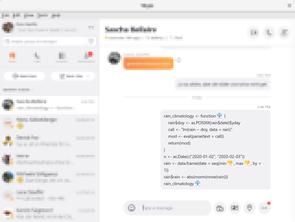
As for yourself, you may write R markdown documents to help out friends and colleagues, or to send a quick update to your boss or advisor. In my old days I (Reto) typically copy-pasted R code into e-mails or skype. That works OKish for simple things with only a hand full lines of code, however, it is hard to structure more complex code/solutions properly. In addition: if the client of your opponent converted everything into html, some parts of the code may be converted into smilies, beer mugs, or flamingos. Don’t believe me?
Try to send this message via skype:
rain_climatology <- function(rain) {
    rain$doy <- as.POSIXlt(rain$date)$yday
    call <- "lm(rain ~ doy, data = rain)"
    mod <- eval(parse(text = call))
    return(mod)
}
n <- as.Date(c("2020-01-02", "2020-02-03"))
rain <- data.frame(date = seq(min(n), max(n), by = 1))
rain$rain <- abs(rnorm(nrow(rain)))
rain_climatology(rain)
The result is this:
Instead, we could write a short and simple .Rmd file which contains
- The code.
- The result of the code.
- Additional explanations.
- And even some results (plots, tables).
For your job
More ‘advanced’; imagine working with live data which are getting updated every few hours, days, or weeks, and you do have to create a report for your boss. Or: you create a report for yourself to monitor the data. E.g.,:
- Biology: measuring some parameters of a process in the lab (temperature, nutrition, and the corresponding biomass in a test tube).
- Meteorology: live-measurements of the smog concentration in your city.
- Economics: monthly reports of credit/debit balances.
- Marketing: check if your spendings (advertisements) led to the desired result.
- Tourism: monitor the number of bookings/tickets sold for a specific event, hotel, or skiing ressort.
- Sales management: weekly reports of products sold, products in stock, and an analysis if you have to re-order new some products not to run out of stock.
- Web development: monitor the number of visits on your website and the user behaviour.
As you can see, this is not restricted to a specific field of research or industry. Nowadays, data are collected everywhere and dynamic reports (e.g., using R markdown) can be used to analyze these data - and that’s the basis of data science.
R Code Chunks
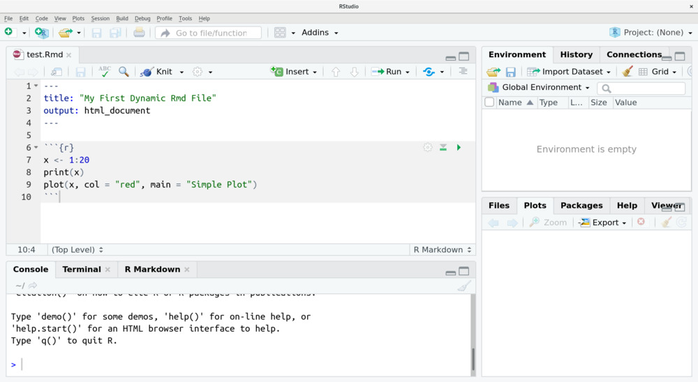
Whenever we create a new R Markdown file in RStudio, RStudio gives us a demo file with some content (shown above) which also contains some R chunks. R chunks are defined as follows:
```{r}
x <- 1:20
print(x)
plot(x, col = "red", main = "Simple Plot")
```
As in pure markdown we open and close a code block with three backticks
(see also Markdown Syntax).
To turn a markdown code block into an R chunk, we additionally have to
set the {r} when opening the block. This tells knitr that this
is code we want to execute. Within the curly braces we set additional
options if needed ({r, ...}). By default:
- The input (code) will be shown in the final document.
- The output (prints) will be shown in the final document.
- In case there is a plot, the figure will also be included.
Exercise 18.1 Let’s try it out. Create a new .Rmd file.
Specify at least a title and the output format in the yml header,
and copy the code chunk shown above into this new .Rmd file.
Feel free to add additional content such as text or titles (headings).
Once you’ve done, save the .Rmd file if you have not yet done it and
knit the document by pressing the “Knit” button.
If everything works as expected, you should end up with an HTML document
which shows the R input (code of the R chunk) and the results - in this
case the result of print() and a simple figure created by plot().
Code Chunk Options
Additional knitr-options can be provided to control the chunks.
These options can be set globally (check ?knitr::opts_knit)
or individually for specific R chunks.
The options are set as key = value pairs within the curly
braces ({r, key = value, key = value, ...}).
The following list shows some of the most important options:
include = FALSE: if set, the chunk is executed, but nothing shows up in the final document. Can be used to prepare data without including it int the output document.echo = FALSE: do not show the input (R code). Default isTRUE.results = "hide": do not show results (e.g., fromprint()).fig.keep = "none": do not include plots.fig.width = X: numeric, width of the resulting plot (in inches).fig.height = X: numeric, height of the resulting plot (in inches).
An example:
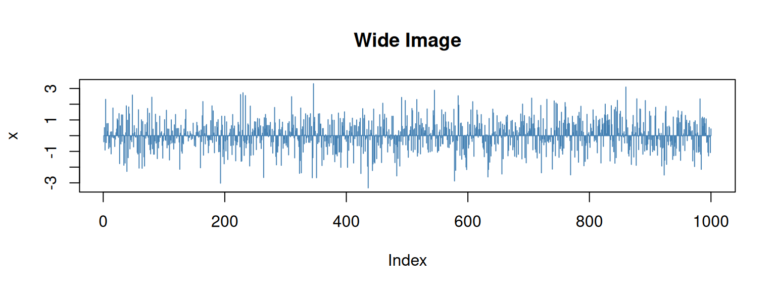
```{r, echo = FALSE, results = "hide", fig.width = 8, fig.height = 3}
# Draw 1000 values from a random distribution
x <- rnorm(1000)
print(x)
# Plot the data
plot(x, type = "h", col = "steelblue",
     main = "Wide Image")
```
This should lead to the result shown below. As you can see,
the R source code (input; echo = FALSE) is not shown, neither the result of
the print() call shows up (output; results = "hide"). All we get at the
end is the plot (format: \(8 \cdot 3\) inches; landscape).
18.3.1 Inline Code
In addition to R code chunks we can also execute R commands “inline”. Inline means “in text” and allows us to dynamically create text. As R code chunks are an extension of markdown code blocks, inline code is an extension of markdown inline code (see Markdown Syntax).
Instead of having three backticks and {r} inline code is defined as follows:
`r paste("Happy", 2020)`The “r” tells knitr that this expression (code) must be executed when knitting the document. We can now use this in the text. As an example: the following line:
**Hy there, we wish you a `r paste("Happy", 2020)`!**… will generate the following: Hy there, we wish you a Happy 2020!
The code within the ticks is executed (paste("Happy", 2020)) and “inserted” into
the text at this specific position.
This can be used to print some numbers in the text (e.g., the current date, or
the maximum of a specific variable), or more complex. With some logic we could
adjust the text dynamically and generate data-dependent output.
As an example, let’s imagine we have a weather forecast for tomorrow and, depending on the forecasted temperature and sunshine duration, the text output should be different. Therefore, we could write a small function which we can use in combination with inline code:
weather_forecast <- function(temperature, sunshine) {
    if (temperature < 0 & sunshine > 5) {
        res <- paste("Tomorrow will be very cold with a temperature of only",
                     temperature, "degrees Celsius. However, with ", sunshine,
                     "hours of sun it is worth to go outside!")
    } else if (temperature < 0) {
        res <- paste("Cold and only little sun expected for tomorrow.",
                     "Suggestion: stay at home!")
    } else if (sunshine < 5) {
        res <- paste("With", temperature, "degrees Celsius it will be warm tomorrow,",
                     "however, with only", sunshine, "hours of sun it sounds like a couch day.")
    } else {
        res <- paste("Warm an sunny! With", temperature, "degrees Celsius and up to",
                     sunshine, "hours of sunshine it will be a nice day.")
    }
    return(res)
}
We can now use the function inline (calling weather_forecast(-9.3, 0.2) or
weather_forecast(8.3, 6.2), …). Two examples:
Tomorrows weather forecast: Cold and only little sun expected for tomorrow. Suggestion: stay at home!
Tomorrows weather forecast: Warm an sunny! With 8.3 degrees Celsius and up to 6.2 hours of sunshine it will be a nice day.
18.3.2 Tables
knitr comes with a function called kable() to create
html tables in the output. The input to kable() is typically
a matrix or data frame. Let’s use the old faithful data set
to demonstrate this feature:
##   eruptions waiting
## 1     3.600      79
## 2     1.800      54
## 3     3.333      74
## 4     2.283      62
## 5     4.533      85
## 6     2.883      55
Instead of printing the data frame as shown above, we can
call kable(faithful) within the R chunk.
| eruptions | waiting |
|---|---|
| 3.600 | 79 |
| 1.800 | 54 |
| 3.333 | 74 |
| 2.283 | 62 |
| 4.533 | 85 |
| 2.883 | 55 |
Typically you suppress the input (R chunk options; set echo = FALSE) to
only show the table, but not the code. One problem with knitr::kable(): if
you have dozends of observations, the resulting table will ge very large.
Thus, this should be used for summary tables or results, and not to show
large data frames or matrices. Other contributed packages (e.g.,
DT) provide more functionality to create tables.
Just as a teaser: