Chapter 5 Matrices
In the Vectors chapter we have learned about the atomic vectors and that they build the base for more complex objects. The next level of complexity are arrays and matrices. An array is a multi-dimensional extension of a vector. In the special case that the array has only two dimensions, this array is also called a matrix.
We will only work with matrices and not with arrays of higher dimensions. However, the step towards higher-dimensional arrays is simple once we know how to handle matrices.
5.1 Matrix introduction
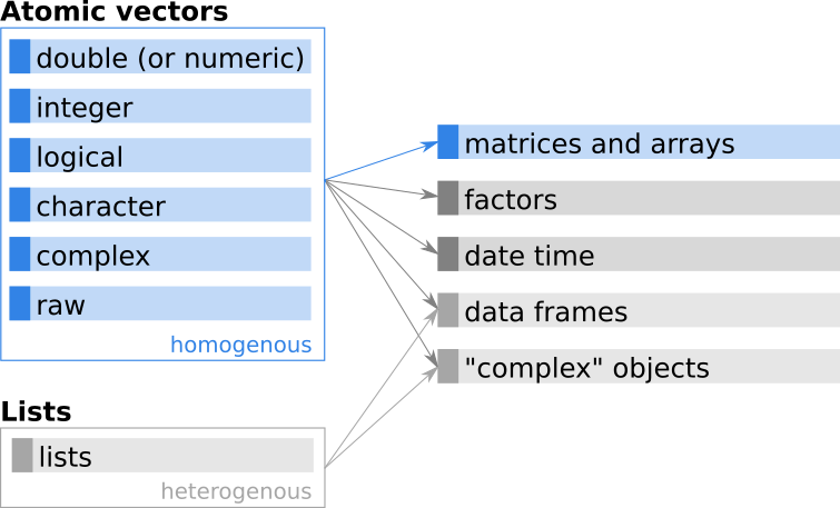
Figure 5.1: Simplified relationship between atomic vectors and matrices/arrays.
While a vector is a (long) sequence of values, a matrix is a two-dimensional rectangular object with values. Important aspects of matrices in R:
- Arrays are based on atomic vectors.
- A matrix is a special array with two dimensions.
- Matrices can only contain data of one type (like vectors).
- Matrices always also have a length (number of elements).
- In addition to vectors, matrices have an additional dimension attribute
(
dim()) which vectors don’t have. - As vectors, matrices can have names (row and column names; optional attribute).
Most of you should be familiar with matrices
from mathematics, where a matrix x with 3 rows and 4 columns is defined as:
\[ x = \left(\begin{array}{cc} x_{11} & x_{12} & x_{13} & x_{14} \\ x_{21} & x_{22} & x_{23} & x_{24} \\ x_{31} & x_{32} & x_{33} & x_{34} \\ \end{array}\right) \]
The matrix \(x\) consists of three rows (\(i \in \{1, 2, 3\}\)) and four columns (\(j \in \{1, 2, 3, 4\}\)), wherefore this matrix is of dimension \(3 \times 4\). The individual elements of the matrix are denoted as \(x_{\color{blue}{i}\color{red}{j}}\) – where the first subscript is (always) the row-index, the second one the column-index. The element in the second row (\(\color{blue}{i = 2}\)) and fourth column (\(\color{red}{j = 4}\)) is thus \(x_{\color{blue}{2}\color{red}{4}}\). In R, matrices follow the same design. Let us re-write the matrix above to:
\[ \text{x} = \left(\begin{array}{cccc} \text{x}[{\color{blue}{1}}, {\color{red}{1}}] & \text{x}[{\color{blue}{1}}, {\color{red}{2}}] & {\text{x}[\color{blue}{1}}, {\color{red}{3}}] & {\text{x}[\color{blue}{1}}, {\color{red}{4}}] \\ \text{x}[{\color{blue}{2}}, {\color{red}{1}}] & \text{x}[{\color{blue}{2}}, {\color{red}{2}}] & {\text{x}[\color{blue}{2}}, {\color{red}{3}}] & {\text{x}[\color{blue}{2}}, {\color{red}{4}}] \\ \text{x}[{\color{blue}{3}}, {\color{red}{1}}] & \text{x}[{\color{blue}{3}}, {\color{red}{2}}] & {\text{x}[\color{blue}{3}}, {\color{red}{3}}] & {\text{x}[\color{blue}{3}}, {\color{red}{4}}] \\ \end{array}\right) \]
The blue numbers correspond to the row indices (thus always \(1\) for the top row, \(2\) for the second row, …), the red numbers denote the indices of the columns (\(1\) leftmost column, …, \(4\) rightmost column in this example).
Let us have a look at how R displays matrices. The following output
shows a \(3 \times 4\) matrix (as above) with missing values (all elements are NA)
and how R displays/prints the matrix.
##      [,1] [,2] [,3] [,4]
## [1,]   NA   NA   NA   NA
## [2,]   NA   NA   NA   NA
## [3,]   NA   NA   NA   NA
Again, the information in square brackets ([1,] or [,3]) is not part of the
matrix itself, but helps you to read the output. On the left side you can see
the indicator/number of the rows ([1,] = first row, [2,] = second row,
[3,] = third row), while on top you can see the same for the columns ([,1]
= first column, … [,4] = fourth column).
We will come back to this later on when subsetting matrices.
5.2 Creating matrices
Matrices can be created using the matrix() function. According to the R
documentation the usage of the matrix() function (see ?matrix or
help("matrix")) is as follows:
matrix(data = NA, nrow = 1, ncol = 1, byrow = FALSE, dimnames = NULL)data: a data vector (defaultNA)nrow: desired number of rows (first dimension, ‘top down’; default1).ncol: desired number of columns (second dimension, ‘left to right’; default1).byrow: logical, whether or not to fill by row (defaultFALSE; fill by column).dimnames: optional list of length 2 with row names and column names (defaultNULL).
Note that some of the arguments have “defaults”. These default values are used if you do not explicitly change them – we will learn about function defaults in the next chapter (Functions).
To create a matrix containing a constant value of 999L (data = 999L) with two rows (nrow = 2)
and three columns (ncol = 3) we call:
##      [,1] [,2] [,3]
## [1,]  999  999  999
## [2,]  999  999  999
We can now check the dimension of the object using dim(). dim() always
returns an integer vector with two elements (for matrices). The first
corresponds to the number of rows (first dimension), the second entry to the
number of columns (second dimension). In combination with subsetting we can get
the number of rows using:
## [1] 2 3## number of rows number of columns
## 2 3Alternatively, we can make use of the two convenience functions nrow() and
ncol(). The return of these two functions is a single integer with either
the number of rows, or number of columns.
## [1] 2## [1] 3As mentioned earlier, matrices always have a length. Matrices are based
on atomic vectors, the length is nothing else than the number of elements of the
underlying vector. When checking the matrix x from above, which is of dimension
\(2 \times 3\) we get \(6\) as the matrix (and thus the underlying atomic vector)
contain \(6\) elements. This is nothing else than the number of rows times the
number of columns.
## [1] 6## [1] 6Matrix-to-vector
As all matrices (and arrays) are based on vectors, we can use explicit coercion
to convert them back and forth. Let us take our matrix x and explicit coercion
to convert it into a vector (as.vector()):
## [1] 999 999 999 999 999 999## [1] 6As shown, this returns to us the vector on which matrix x is based.
This is, of course, a vector of length \(6\) (thus length(x) == length(y)).
This vector can be used to create the matrix again by calling matrix() using
vector y as our argument for data.
##      [,1] [,2] [,3]
## [1,]  999  999  999
## [2,]  999  999  999
Type of data
Matrices (as vectors) can only contain data of one type. We
can create numeric matrices, integer matrices, character matrices, and logical
matrices by adding the corresponding values in the data argument when
creating a matrix.
The following four matrices are all based on vectors of different types (double, integer, character, and logical).
x1 <- matrix(seq(0, 4.5, length.out = 9), nrow = 3)    # double
x2 <- matrix(1:9, nrow = 3)                            # integer
x3 <- matrix(LETTERS[1:9], nrow = 3)                   # character
x4 <- matrix(TRUE, nrow = 3, ncol = 3)                 # logical
Investigate the objects: We can check the type of the objects using the
is.*() functions. Take one of the examples above and try it yourself:
| is.double() | is.numeric() | is.integer() | is.character() | is.logical() | |
|---|---|---|---|---|---|
| x1 | TRUE | TRUE | FALSE | FALSE | FALSE |
| x2 | FALSE | TRUE | TRUE | FALSE | FALSE |
| x3 | FALSE | FALSE | FALSE | TRUE | FALSE |
| x4 | FALSE | FALSE | FALSE | FALSE | TRUE |
Exercise 5.1 Try to create the following matrices. To do so, we need to specify data,
the number of rows, and the number of columns.
- A matrix of dimension \(5 \times 5\) which contains
5L(integer) everywhere. - A matrix of dimension \(10 \times 1\) which contains
-100(numeric) everywhere. - Check that the class of your result is
c("matrix", "array"). - Use
is.matrix(),is.double(),is.integer(), andis.numeric()to check the type of the data of the matrix.
Solution. Matrix \(5 \times 5\): The dimension should be \(5 \times 5\), thus we have to
set nrow = 5 and ncol = 5. In addition, we need to specify the data. Instead
of using the default (data = NA) we simply use data = 5L.
##      [,1] [,2] [,3] [,4] [,5]
## [1,]    5    5    5    5    5
## [2,]    5    5    5    5    5
## [3,]    5    5    5    5    5
## [4,]    5    5    5    5    5
## [5,]    5    5    5    5    5
Our matrix (\(5 \times 5\)) has 25 elements, but we only specified
one single integer in data. What happens is that R recycles
this element as often as needed (the same happens with the default data = NA).
In this case it recycles 5L 25 times for each entry in the matrix.
We could also generate a vector which contains 5L 25 times (remember the
rep() function to replicate elements) which yields the very same result.
##      [,1] [,2] [,3] [,4] [,5]
## [1,]    5    5    5    5    5
## [2,]    5    5    5    5    5
## [3,]    5    5    5    5    5
## [4,]    5    5    5    5    5
## [5,]    5    5    5    5    5
Checking class and dimension:
## [1] "matrix" "array"## [1] 5 5The object x should be an integer matrix. Let us check this
using the corresponding is.*() functions:
c("is.matrix"  = is.matrix(x),
  "is.integer" = is.integer(x),
  "is.double"  = is.double(x),
  "is.numeric" = is.numeric(x))
## is.matrix is.integer is.double is.numeric
## TRUE TRUE FALSE TRUEAs for vectors, integers are both, integer and numeric (as we can use arithmetic). However, an integer is not a double (floating point numeric value).
Matrix of dimension \(10 \times 1\): Very similar to the first exercise. All we have to do is to take care which dimension corresponds to what.
A \(10 \times 1\) matrix has 10 rows and one column, thus we need to call:
##       [,1]
##  [1,] -100
##  [2,] -100
##  [3,] -100
##  [4,] -100
##  [5,] -100
##  [6,] -100
##  [7,] -100
##  [8,] -100
##  [9,] -100
## [10,] -100
Perform the same checks as above to see that everything is fine.
## [1] "matrix" "array"## [1] 10 1c("is.matrix" = is.matrix(x),
"is.integer" = is.integer(x),
"is.double" = is.double(x),
"is.numeric" = is.numeric(x))## is.matrix is.integer is.double is.numeric
## TRUE FALSE TRUE TRUE100 (without the L suffix) defines a floating point number (100.00000).
Thus it is both, numeric and double, but not integer.
Order of elements
Let us have a closer look at x2, the integer matrix from above,
and how the elements of the vector end up in the matrix.
##      [,1] [,2] [,3]
## [1,]    1    4    7
## [2,]    2    5    8
## [3,]    3    6    9
This matrix is of dimension \(3 \times 3\). But how does R know how big the
matrix must be? If we check the command we can see that we provide an integer
vector with 9 elements, and ask for a matrix with 3 rows (nrow = 3). There
is only one way to fulfill the requirements: creating a \(3 \times 3\) matrix.
When we look at the output above we can also see how the values have been
filled in. At first, the leftmost column has been filled (with 1, 2, and
3), then the second (4, 5, 6), and last but not least the third column
(7, 8, 9). This is called filled by column. The image below shows a
sketch of what is happening here:
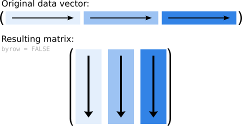
Figure 5.2: Sketch of how the data are added to a matrix (by column; default).
This is the default behavior of matrix() as the input argument byrow is set to FALSE.
We can change this by setting byrow = TRUE. Instead of filling in the data by column,
the top row is now filled first, followed by the second, and so far and so on.
Accordingly our matrix looks different now:
##      [,1] [,2] [,3]
## [1,]    1    2    3
## [2,]    4    5    6
## [3,]    7    8    9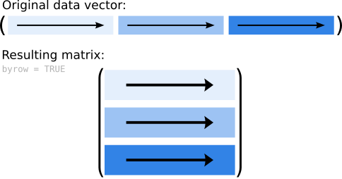
Figure 5.3: Sketch of how the data are added to a matrix when setting byrow = TRUE.
Note: This changes the order of the elements in the underlying vector.
The underlying vector is always by column. When using byrow = TRUE the
matrix (and thus also the underlying vector) get re-ordered. Let us check:
##      [,1] [,2] [,3]
## [1,]    1    2    3
## [2,]    4    5    6
## [3,] 7 8 9## [1] 1 4 7 2 5 8 3 6 9The transposed of a matrix: Just a side note; if we have a quadratic matrix
(same number of rows and columns) the results of matrix() once with byrow = TRUE and once with byrow = FALSE results in two matrices where one is the
transposed of the other one.
##      [,1] [,2] [,3]
## [1,]    1    4    7
## [2,]    2    5    8
## [3,] 3 6 9## [,1] [,2] [,3]
## [1,] 1 2 3
## [2,] 4 5 6
## [3,] 7 8 9This is no longer true for rectangular matrices. To transpose matrices, a function
t() (transpose) can be used which (in this case) yields the same result (compare to x2).
##      [,1] [,2] [,3]
## [1,]    1    2    3
## [2,]    4    5    6
## [3,] 7 8 9Exercise 5.2 Create some matrices given a data vector created by replicate (see Replicating elements from the previous chapter).
Below you can see the three data vectors (data_A, data_B, data_C)
and three matrices (A, B, C).
data_A <- rep(c(-1, 0, 1), 5)                        # For matrix A
data_B <- rep(c(-3, -2, -1, 0, 1, 2, 3), each = 3)   # For matrix B
data_C <- rep(c(1, 0, 0, 0, 0), length.out = 16)     # For matrix C
And this is how the matrices should look at the end:
##      [,1] [,2] [,3] [,4] [,5]
## [1,]   -1   -1   -1   -1   -1
## [2,]    0    0    0    0    0
## [3,] 1 1 1 1 1## [,1] [,2] [,3]
## [1,] -3 -3 -3
## [2,] -2 -2 -2
## [3,] -1 -1 -1
## [4,] 0 0 0
## [5,] 1 1 1
## [6,] 2 2 2
## [7,] 3 3 3## [,1] [,2] [,3] [,4]
## [1,] 1 0 0 0
## [2,] 0 1 0 0
## [3,] 0 0 1 0
## [4,] 0 0 0 1The exercise: Use the function matrix() and the three ‘data vectors’
to create the three matrices printed above by setting the correct arguments
when calling matrix().
Solution. Matrix A: For data_A we repeat a vector of length 3 (c(-1, 0, 1))
which results in a vector of length 15. Matrix A has 3 rows and
5 columns (thus 15 elements). To create A we need to call matrix() with
(i) data = data_A and either (ii) nrow = 3 or (iii) ncol = 5.
When rows or columns are given, the dimension of the matrix is already defined.
However, we can, of course, also set both (nrow and ncol).
A <- matrix(data = data_A, nrow = 3)
A <- matrix(data = data_A, ncol = 5)
A <- matrix(data = data_A, nrow = 3, ncol = 5)Matrix B: The replication command (when data_B is generated) repeats
each element three times. Thus, our vector looks something like c(-3, -3, -3, -2, -2, -2, ...).
Again, the length matches the number of elements of the matrix, thus it is enough if we only
define one of the two arguments nrow and ncol.
The important part here: each row contains one constant value. Given our vector data_B the
elements have to be filled in by row to get the correct result. Therefore we need to set
byrow = TRUE.
##      [,1] [,2] [,3]
## [1,]   -3   -3   -3
## [2,]   -2   -2   -2
## [3,]   -1   -1   -1
## [4,]    0    0    0
## [5,]    1    1    1
## [6,]    2    2    2
## [7,] 3 3 3Matrix C: The rep() function repeats c(1, 0, 0, 0, 0) up to a length of 16
elements, just enough to fill our \(4 \times 4\) matrix. This special vector yields
a diagonal matrix (a matrix where the diagonal from top left to bottom right) contains
1 while all other elements are 0. It does not even matter if we fill in the elements
by row, or by column, we will get the very same result. Two possible ways to solve this:
##      [,1] [,2] [,3] [,4]
## [1,]    1    0    0    0
## [2,]    0    1    0    0
## [3,]    0    0    1    0
## [4,] 0 0 0 1## [,1] [,2] [,3] [,4]
## [1,] 1 0 0 0
## [2,] 0 1 0 0
## [3,] 0 0 1 0
## [4,] 0 0 0 15.3 Matrix functions
As for vectors a series of functions exist to work with matrices. The following list is not a complete list, but contains some useful functions for matrices:
| Function | Description |
|---|---|
head() |
Return first few rows. |
tail() |
Return last few rows. |
summary(x) |
Numerical summary of the matrix (column-wise). |
rbind() |
Combine objects ‘by row’. |
cbind() |
Combine objects ‘by column’. |
order() |
Allows to sort matrices. |
... |
Many more functions exist. |
As matrices are based on vectors, we can also use all functions from the table shown
in Vector functions
like e.g., get the minimum (min()), calculate the logarithm of all elements (log()),
or check elements (e.g., all(x > 0)).
Try this yourself!
Exercise 5.3 Generate matrix: We will work with a fairly large matrix called mat with
random values. Thus, to get the same results as in this book, we need to set a
random seed first. To make the output a bit cleaner, all random values are
rounded to one digit after the coma (round(..., digits = 1)).
## [1] 20 5The matrix is of dimension \(20 \times 5\) and thus takes up quite some space when we print the matrix. Instead:
- Call
head(mat)andhead(mat, n = 2)to get the first 6 (default) or 2 rows only. - Call
tail(mat)andtail(mat, n = 3)to get the last 6 or 3 rows. - Call
summary(mat)and try to interpret the output. Do you see what happens?
In a second step try to answer the following questions:
- Get the largest and smallest value in the matrix (minimum and maximum).
- What is the arithmetic mean (average), what the standard deviation of the entire matrix?
- What is the sum of the entire matrix
mat?
Solution. Head and tail: As for vectors, head() and tail() only show parts of the object, in case of matrices
the first/last few rows.
##      [,1] [,2] [,3] [,4] [,5]
## [1,] -0.6  0.9 -0.2  2.4 -0.6
## [2,]  0.2  0.8 -0.3  0.0 -0.1
## [3,] -0.8  0.1  0.7  0.7  1.2
## [4,]  1.6 -2.0  0.6  0.0 -1.5
## [5,]  0.3  0.6 -0.7 -0.7  0.6
## [6,] -0.8 -0.1 -0.7 0.2 0.3## [,1] [,2] [,3] [,4] [,5]
## [1,] -0.6 0.9 -0.2 2.4 -0.6
## [2,] 0.2 0.8 -0.3 0.0 -0.1## [,1] [,2] [,3] [,4] [,5]
## [15,] 1.1 -1.4 1.4 -1.3 1.6
## [16,] 0.0 -0.4 2.0 0.3 0.6
## [17,] 0.0 -0.4 -0.4 -0.4 -1.3
## [18,] 0.9 -0.1 -1.0 0.0 -0.6
## [19,] 0.8 1.1 0.6 0.1 -1.2
## [20,] 0.6 0.8 -0.1 -0.6 -0.5## [,1] [,2] [,3] [,4] [,5]
## [18,] 0.9 -0.1 -1.0 0.0 -0.6
## [19,] 0.8 1.1 0.6 0.1 -1.2
## [20,] 0.6 0.8 -0.1 -0.6 -0.5This is often useful to see what an object (matrices, data frames) contain without printing the entire matrix onto your screen (which might take quite a while if you have large objects).
Numeric summary: The function summary() applied to a matrix gives us the
numerical summary as for vectors, but for each column individually.
##        V1               V2               V3               V4
##  Min.   :-2.200   Min.   :-2.000   Min.   :-1.100   Min.   :-1.800
##  1st Qu.:-0.375   1st Qu.:-0.400   1st Qu.:-0.450   1st Qu.:-0.625
##  Median : 0.350   Median :-0.100   Median : 0.100   Median : 0.050
##  Mean   : 0.195   Mean   :-0.015   Mean   : 0.145   Mean   : 0.115
##  3rd Qu.: 0.725   3rd Qu.: 0.650   3rd Qu.: 0.625   3rd Qu.: 0.525
##  Max.   : 1.600   Max.   : 1.400   Max.   : 2.000   Max.   : 2.400
##        V5
##  Min.   :-1.500
##  1st Qu.:-0.525
##  Median : 0.300
##  Mean   : 0.130
##  3rd Qu.: 0.800
##  Max.   : 1.600
The names on top (V1, V2, …) simply mean “variable 1”, “variable 2”, etc. In case
we have a named matrix (we will come back to this in the next subchapter) the original
names would be shown. For each column we get the minimum, median, mean, and maximum, plus
the first and third quartile. In case there would be missing values, the number of NAs would
also be shown (very same as for vectors).
Minimum and maximum: To get the minimum and maximum we simply call min() and max().
Note: in case the matrix contains missing values, we might need min(..., na.rm = TRUE).
## minimum maximum
##    -2.2     2.4
Mean and standard deviation: In the same way we can apply a series of mathematical
functions, here mean() and sd() (again, we might take care of missing values):
##    arithmetic mean standard deviation
##           0.114000           0.900395
Given that our matrix is based on random values from the standard normal distribution, the mean should be close to 0 and the standard deviation close to 1. Looks good!
Sum: Function sum() returns the sum of all elements.
## [1] 11.45.4 Mathematical operations
Matrices are often used for arithmetic (mathematics; working with numbers) to solve mathematical problems such as solving systems of linear equations, estimate regression models, and many more. The following sections give an brief introduction on mathematical operations in combination with matrices.
Matrices and scalars
One of the most simple operations is to work with a matrix and a scalar (single numeric value). In principle, all basic arithmetic operations work element-wise as for vectors (see Vectors: Mathematical operations).
As for vectors we can perform e.g., addition or multiplication as follows:
##      [,1] [,2]
## [1,]    1    3
## [2,] 2 4## [,1] [,2]
## [1,] 3 5
## [2,] 4 6## [,1] [,2]
## [1,] 1.5 4.5
## [2,] 3.0 6.0The same is true for all other operations including +, -, *, /, ^,
%%, sin(), cos(), and many more (see Vectors: Mathematical operations).
The operation is applied element-by-element, the result of these operations
is always a matrix of the same dimension with the same attributes.
Matrices and Vectors
Beside using a matrix and a scalar, we can perform arithmetic using a matrix and a vector. What happens if we e.g., multiply a matrix of dimension \(2 \times 2\) with a vector of length \(2\)?
##      [,1] [,2]
## [1,]   10   30
## [2,]  200  400
The matrix has \(2 \times 2 = 4\) elements while the vector is shorter and contains only \(2\) elements. Thus, R recycles (re-uses) the vector elements to be able to perform the calculations.
For a better understanding, the following code chunk illustrates what happens:
R spans up a new matrix based on vector y which matches the dimension of x.
We can manually do the same by calling:
##      [,1] [,2]
## [1,]   10   10
## [2,]  100  100
The matrix above (which evolves from our vector y) now contains c(10, 100) twice (to match the dimension)
and is then multiplied with matrix x.
##      [,1] [,2]
## [1,]   10   30
## [2,]  200  400
As you can see, we end up with the same result as before using x * y.
Matrices and matrices
In the same way, simple ‘matrix and matrix’ operations work. When two matrices are of the same dimension, we can use basic element-wise arithmetic operations.
##      [,1] [,2]
## [1,]    1    3
## [2,] 2 4## [,1] [,2]
## [1,] 10 30
## [2,] 20 40## [,1] [,2]
## [1,] 11 33
## [2,] 22 44As in the previous sub-chapters the operation (addition) is done element-by-element
(\(1 + 10 = 11\), \(2 + 20 = 22\), etc.), the result is a matrix of the same size
with the same attributes as the first element (x)
The same, of course, works for other mathematical operations like division or taking x^y.
##      [,1] [,2]
## [1,]  0.1  0.1
## [2,] 0.1 0.1## [,1] [,2]
## [1,] 1 2.058911e+14
## [2,] 1048576 1.208926e+24More matrix arithmetic
Besides simple arithmetic, R comes with a wide range of functions for mathematical tasks and can do ‘all’ you need. These functions are not part of “Introduction to Programming with R” but keep in mind that all can be done using base R. The following list is incomplete, but gives an idea what we can do beyond the content of this introduction.
| Command | Description |
|---|---|
t(x) |
Transpose x. |
diag(x), diag(3L) |
Diagonal elements of x. |
x %*% y |
Matrix multiplication (inner product). |
solve(x) |
Inverse of x. |
solve(a, b) |
Solve system of linear equations. |
crossprod(x, y) |
Cross product. |
outer(x, y), x %o% y |
Outer product. |
kronecker(x, y) |
Kronecker product. |
det(x) |
Determinant. |
qr(x) |
QR decomposition |
chol(x) |
Cholesky decomposition |
... |
… and many more |
For those interested in linear algebra/advanced mathematical topics using R, you may be want to check the following sources:
- See
?matmultorhelp("matmult")for more details - Matrix algebra tutorial with R solution from “198812 VU Computer Programming Prerequisites” by the DiSC: Session 2, Session 5
- https://www.math.uh.edu/~jmorgan/Math6397/day13/LinearAlgebraR-Handout.pdf
- https://www.amazon.com/Hands-On-Matrix-Algebra-Using-Applications/dp/9814313696
5.5 Matrix attributes
As we know from the Vectors chapter and the first part
of this chapter, all object have some
mandatory attributes (such as the class), and can have additional ones.
As mentioned earlier (see Matrices) matrices
always have a specific class (c("matrix", "array")), a length, and a dimension attribute.
We can again use the attributes() function to check the attributes
of a plain matrix.
## $dim
## [1] 10  2
Dimension
Every matrix, even a plain matrix, always has the dimension attribute which
we can access with the functions dim(), nrow(), and ncol().
dim() returns an integer vector of length \(2\) (for matrices) where the first
element corresponds to the first dimension (number of rows), the second to the
second dimension (number of columns). For convenience, nrow() and ncol() return
a single integer for the first or second dimension, respectively.
## [1] 10 2## number of rows number of columns
## 10 2Just a small excursion on how we could also generate matrices. Please note: that
this is not the preferred way to do it, but it is possible and demonstrates what
happens. Imagine we have the following simple vector data with 25 random values:
set.seed(789) # Pseudo-random-numbers
# 25 random values from a normal distribution, rounded
data <- round(rnorm(25), 3)
data
## [1] 0.524 -2.261 -0.020 0.183 -0.361 -0.484 -0.666 -0.174 -1.011 0.740
## [11] -0.402 -1.003 -0.178 -0.488 0.928 -0.774 0.423 -0.607 0.209 -0.777
## [21] -0.702 0.683 -0.858 0.368 -1.430## [1] 25## NULLdata is a numeric vector which comes, as we have learned in chapter
Vectors, with one single attribute
“length” but has no dimension attribute.
What if we would set one? Let us add an additional dimension attribute to
data (dimension c(5L, 5L), \(5\) rows and \(5\) columns).
## [1] 5 5Like for names() we can, technically, add a dimension attribute by
using dim(data) <- c(..., ...). As vectors don’t have dimensions, R
automatically assumes that this must now be a matrix of this specific dimension.
## [1] TRUE## [,1] [,2] [,3] [,4] [,5]
## [1,] 0.524 -0.484 -0.402 -0.774 -0.702
## [2,] -2.261 -0.666 -1.003 0.423 0.683
## [3,] -0.020 -0.174 -0.178 -0.607 -0.858
## [4,] 0.183 -1.011 -0.488 0.209 0.368
## [5,] -0.361 0.740 0.928 -0.777 -1.430This nicely demonstrates that the main difference between a vector and a matrix is the dimension.
Length and type
As all matrices are based on (atomic) vectors, all matrices also have a length and a specific type.
- Length of a matrix: The length is simply the total number of elements of the matrix, or the length of the underlying atomic vector.
- Type of data: While
class()tells us that a matrix is of class matrix/array,typeof()can be used to get the type of the data itself (see Vectors).
x <- matrix(c(1L, 2L, 3L, 4L), ncol = 2)
length(x) == nrow(x) * ncol(x)    # Length gives us the number of elements
## [1] TRUE## [1] "matrix" "array"## [1] "integer"As for vectors a series of is.*() can be used to check the object. The two new
ones below are is.vector() and is.matrix() to see if our object is a vector or a matrix.
In addition, we can use is.*() to check if the object (matrix) is of a specific type.
c("is.matrix"    = is.matrix(x),
  "is.vector"    = is.vector(x),
  "is.numeric"   = is.numeric(x),
  "is.integer"   = is.integer(x),
  "is.logical"   = is.logical(x),
  "is.character" = is.character(x))
## is.matrix is.vector is.numeric is.integer is.logical is.character
## TRUE FALSE TRUE TRUE FALSE FALSEDimension names
As for vectors, one optional argument of matrices are ‘names’. While we use
the function names() when working with vectors (see Vector
attributes),
this no longer works for matrices as they are two-dimensional.
Instead, we have row names and column names (or in general: dimension names).
rownames(): names of the rows of a matrix.colnames(): names of columns of a matrix.dimnames(): returns all dimension names (as a list; works for all arrays).
These two functions rownames() and colnames() can be used in the same way
as names() for vectors to either retrieve (get) or add (set) the names
of the rows and columns of a matrix.
Let us start with an unnamed (plain) matrix x:
##      [,1] [,2] [,3]
## [1,]    1    4    7
## [2,]    2    5    8
## [3,]    3    6    9
When checking the attributes of the object, we can see that no dimension names are returned.
The same is true when calling rownames(), colnames(), or dimnames(): we get NULL as a result
(empty object; no dimensions specified).
## $dim
## [1] 3 3## NULL## NULL## NULLrownames() and colnames() allow us to add row names and/or column names
to this matrix. Let us add some simple names similar to what you know from
Microsoft Excel or comparable spreadsheet applications.
When printing the matrix we see that all our rows and columns are now named:
##       Col A Col B Col C
## Row 1     1     4     7
## Row 2     2     5     8
## Row 3     3     6     9
Once set, we can get these names by using the two functions again.
Note: Row names and column names are always characters, wherefore
rownames() and colnames() always return character vectors (or NULL if no
names specified).
## [1] "Row 1" "Row 2" "Row 3"## [1] "Col A" "Col B" "Col C"## class type length
## "character" "character" "3"Alternatively we could use dimnames() which returns all dimension names at
the same time. dimnames() returns an object of class "list" (more about
lists in the chapter Lists & data frames)
of length two (for matrices) where each element in the list itself is a character
vector – the very same as rownames() and colnames() return.
## [[1]]
## [1] "Row 1" "Row 2" "Row 3"
##
## [[2]]
## [1] "Col A" "Col B" "Col C"
The same can be seen if we call attributes() again on this named matrix. In addition
to the dimension attribute (dim) we now have a second attribute dimnames stored in
our object x.
## $dim
## [1] 3 3
##
## $dimnames
## $dimnames[[1]]
## [1] "Row 1" "Row 2" "Row 3"
##
## $dimnames[[2]]
## [1] "Col A" "Col B" "Col C"
Changing dimension names
At any time we can use rownames() and colnames() to change (or overwrite)
existing names. Let us take the matrix from above – instead of having Col A, Col B, and Col C
we would like to have first, second, and third. This can be achieved by assigning a
vector with our new names to colnames(x).
##       first secon third
## Row 1     1     4     7
## Row 2     2     5     8
## Row 3     3     6     9
Oh dear! I have made a typo (secon instead of second). To fix this, we could (of course)
overwrite all three column names again. However, there is a smarter way to do this.
We only want to change the name of the second column as the other two are correct. As we have learned in the Subsetting vectors chapter we can access specific elements of a vector using the squared brackets. We can do the same here. To only get the second column name we call:
## [1] "secon"The same can be used to only set the second column name by doing as follows:
##       first second third
## Row 1     1      4     7
## Row 2     2      5     8
## Row 3     3      6     9
Problem solved. This can be very handy, especially when you have larger matrices (or other large objects with names). Instead of re-specifying all names (and yes, you will mess it up) we simply replace the one which is inappropriate or wrong.
Exercise 5.4 The code chunk below can be used to create the matrix used in this exercise, simply
copy & paste the code into your RStudio to create the object cereals.
cereals <- structure(c(431.87, 284.33, 621.44, 95.01, 106.03, 102.45, 475.96,
                       297.85, 616.25, 102.93, 84.13, 117.74, 440.12, 313.61, 617.93,
                       109.33, 117.78, 131.14),
                     .Dim = c(6L, 3L), .Dimnames = list(c("United States",
                       "India", "China", "Indonesia",
                        "Braziiil Ole Ole", "Russian Federation"),
                       c("2015", "2016", "in 2017")))
cereals
## 2015 2016 in 2017
## United States 431.87 475.96 440.12
## India 284.33 297.85 313.61
## China 621.44 616.25 617.93
## Indonesia 95.01 102.93 109.33
## Braziiil Ole Ole 106.03 84.13 117.78
## Russian Federation 102.45 117.74 131.14The matrix contains data about the production of cereals over three years for six countries in metric gigatons (The World Bank).
Exercise: Try to do the following:
- Check that the object
cerealsis a matrix. - Extract the dimension (size) from the matrix.
- Extract the row names and column names such that you get a character vector for both dimensions. Store it on a new object and check if it is a character vector and that the length of the vectors are identical with the dimension of the matrix.
- Unfortunately something went wrong with the naming of the rows and columns. Please
correct/fix these mistakes.
- The third column should be called
"2017"not"in 2017". - “
Braziiil Ole Ole” should be “Brazil” only.
- The third column should be called
Solution. Check class: To check that the object is a matrix we can use is.matrix().
## [1] TRUEExtract dimension: This can be done by either using dim() or nrow() and ncol().
## [1] 6 3## [1] 6## [1] 3Extract dimension names: To get the names of the rows and columns we use
rownames() and colnames() and store the return of these functions on two
new objects named rnames and cnames.
We expect that both objects are character vectors.
## [1] TRUE TRUETo check whether or not the length of the two vectors is correct we can compare
the length of rnames and cnames with the actual dimension of the matrix:
## [1] TRUE## [1] TRUECorrecting row and column names: Let us start with the column names. We could do something as follows:
However, you should not do it this way. Imagine we have a matrix with 50 columns. You would need to properly write down all 50 names and it is more than likely that you make a mistake when doing so.
Instead, we only replace the third entry while leaving the other two untouched.
##                 2015   2016   2017
## United States 431.87 475.96 440.12
In this special case we have an integer sequence. Thus, we could also have done it this way (try it yourself):
Note: we assign an integer sequence to colnames() here – but names (all dimension names)
are always characters. R automatically converts 2015:2017 into
a character vector (c("2015", "2016", "2017")).
We can repair the row names (Brazil) the very same way:
Creating named matrices
Instead of creating a plain matrix and adding dimension names in a second step,
we can (similar to what we have seen in the
Vectors chapter)
directly create named matrices using the matrix() function.
The function provides an input argument called dimnames which is NULL by
default (no dimension names specified). We can specify a list containing two
character vectors (dimnames = list(<rownames>, <colnames>)) where the first
entry of this list is a character vector containing the row names (first dimension),
and the second entry in the list is a character vector for the column names.
Keep in mind that the length of the names must match the dimension of the matrix.
(x <- matrix(data = 1:9, nrow = 3, ncol = 3,
             dimnames = list(c("Row 1", "Row 2", "Row 3"),
                             c("Col A", "Col B", "Col C"))))
## Col A Col B Col C
## Row 1 1 4 7
## Row 2 2 5 8
## Row 3 3 6 9The argument to dimnames = ... must always be a list (we will learn more about lists later),
exactly the same what is returned when calling dimnames().
If you only want to specify either row names or column names, the other list element
can simply be set to NULL. Two examples:
# Only row names, column names set to NULL
(x <- matrix(data = 1:9, nrow = 3, ncol = 3,
             dimnames = list(c("Row 1", "Row 2", "Row 3"),
                             NULL)))
## [,1] [,2] [,3]
## Row 1 1 4 7
## Row 2 2 5 8
## Row 3 3 6 9# Only column names, row names set to NULL
(x <- matrix(data = 1:9, nrow = 3, ncol = 3,
dimnames = list(NULL,
c("Col A", "Col B", "Col C"))))## Col A Col B Col C
## [1,] 1 4 7
## [2,] 2 5 8
## [3,] 3 6 95.6 Combine Objects
Multiple vectors
Another way to create matrices in R is to combine two or more vectors (or matrices). Objects can either be row-binded or column-binded (either combine them row-wise or column-wise).
Let us begin with two numeric vectors x and y, both of length 3.
We would like to combine them in one single matrix which we store on a new
object z. To achieve this, we simply have to call cbind(x, y) which column-binds
the two vectors and returns a matrix.
##      x  y
## [1,] 5 11
## [2,] 5 22
## [3,] 5 33
The resulting object z is a matrix of dimension \(3 \times 2\) where
each column contains the data from the two vectors. As x was our first argument when
calling cbind(), x is stored in the first column.
## [1] "matrix" "array"## [1] 3 2cbind() can also be used to combine more than only two objects at the same time,
e.g., cbind(a, b, c, d, e) or similar. rbind() works the very same way except
that the objects are not combined column-wise (“left to right”) but row-wise
(“top down”). A brief example using the same two vectors from above:
##   [,1] [,2] [,3]
## x    5    5    5
## y 11 22 33## [1] 2 3Note: One has to take care about the length of the vectors! Not all
combinations of lengths are allowed. R tries to recycle the vectors to match
the length of the longest vector when you call cbind()/rbind(). In case we
have two vectors of different length (e.g., first vector of length \(10\), second
vector length \(5\)) R will recycle (replicate) the shorter vector to match the
longer one. This only works if the length of the longer vector is a multiple
of the length of the shorter one. If they don’t match you will still get a
matrix, but R will throw a warning that something is fishy
(see exercise below).
Exercise 5.5 Let’s see if we try to column-bind vectors of different lengths. For
simplicity, only use integer vectors of the form 1:2 (vector of length 2) or
1:5 (vector of length 5).
- Try to row-bind and/or column-bind vectors of length:
- 4 and 4
- 8 and 4
- 4 and 8
- 4 and 1
- 5 and 3
- 9 and 10
Solution. For each task (A-F) the vectors will be generated on the fly
and directly used as input arguments to rbind() (works the very same when you use cbind()).
A: Combine 4/4: Nothing special to mention here.
##      [,1] [,2] [,3] [,4]
## [1,]    1    2    3    4
## [2,]    1    2    3    4
B: Combine 8/4: The first vector is of length 8, the second of length 4. To
be able to create a matrix (rectangular form) the second vector needs to be extended
to the same length (length 8). R simply recycles the numbers 1:4 twice to get
a vector of length 8, and this is the result:
##      [,1] [,2] [,3] [,4] [,5] [,6] [,7] [,8]
## [1,]    1    2    3    4    5    6    7    8
## [2,]    1    2    3    4    1    2    3    4
C: Combine 4/8: As for (B), but this time the first vector is shorter why we
see repeating numbers 1:4 in the first row.
##      [,1] [,2] [,3] [,4] [,5] [,6] [,7] [,8]
## [1,]    1    2    3    4    1    2    3    4
## [2,]    1    2    3    4    5    6    7    8
D: Combine 4/1: The first vector is of length 4, the second of length 1. Thus,
the second vector (which is basically just the “number 1”) is repeated 4 times. Thus,
the second row only contains 1’s.
##      [,1] [,2] [,3] [,4]
## [1,]    1    2    3    4
## [2,]    1    1    1    1
E: Combine 5/3: Well, 5 is not divisible by 3 (\(5 / 3 \approx 1.6666667\)). We cannot simply repeat the shorter vector \(N\) times (where N is a natural number) to get a vector of length 5. However, R is still doing the same thing above but warns you that the vectors mismatch. Be aware of these warnings, most often than not this warning means that you are trying to combine data you did not want to combine!
## Warning in rbind(1:5, 1:3): number of columns of result is not a multiple of
## vector length (arg 2)
## [,1] [,2] [,3] [,4] [,5]
## [1,] 1 2 3 4 5
## [2,] 1 2 3 1 2F: Combine 9/10: Of course the same as in (E), 10 is not divisible by 9 wherefore we get the “length mismatch warning” by R.
## Warning in rbind(1:9, 1:10): number of columns of result is not a multiple of
## vector length (arg 1)
## [,1] [,2] [,3] [,4] [,5] [,6] [,7] [,8] [,9] [,10]
## [1,] 1 2 3 4 5 6 7 8 9 1
## [2,] 1 2 3 4 5 6 7 8 9 10Dimension names: When using rbind() or cbind(), R tries
to automatically assign dimension names. In the example above, where we combine
two vectors called x and y R uses the names of these original objects to
add column names (cbind()) or row names (rbind()). If needed we can explicitly
specify them.
We have two vectors participants_age and participants_hgt with information
about age and height of some participants. If we use row-binding or column-binding the names of
these two vectors will be used as dimension names.
# Original vectors
participants_age <- c(  24,   25,   21,   32,   19)
participants_hgt <- c(1.73, 1.62, 1.72, 1.82, 1.71)
# Combine to matrix
rbind(participants_age, participants_hgt)
## [,1] [,2] [,3] [,4] [,5]
## participants_age 24.00 25.00 21.00 32.00 19.00
## participants_hgt 1.73 1.62 1.72 1.82 1.71This works well, but the names are a bit long and unhandy. Instead, we can
specify new names when calling rbind() or cbind() as follows:
##         [,1]  [,2]  [,3]  [,4]  [,5]
## age    24.00 25.00 21.00 32.00 19.00
## height  1.73  1.62  1.72  1.82  1.71
The same works for column binding:
##      age height
## [1,]  24   1.73
## [2,]  25   1.62
## [3,]  21   1.72
## [4,]  32   1.82
## [5,]  19   1.71
Multiple matrices
cbind() and rbind() can also be used to combine matrices. Again, you have
to take care of the dimensions of the matrices and have to decide whether we
would like to combine them row-wise (on top of each other) or
column-wise (from left to right).
Let us use the two matrices x1 and x2, both of dimension \(3 \times 2\).
##      [,1] [,2] [,3] [,4]
## [1,]    1    4  101  104
## [2,]    2    5  102  105
## [3,] 3 6 103 106## [,1] [,2]
## [1,] 1 4
## [2,] 2 5
## [3,] 3 6
## [4,] 101 104
## [5,] 102 105
## [6,] 103 106What differs from row-binding/column-binding two vectors is that no row or
column names are automatically added. The reason is simple: Our matrices (x1,
x2) can have multiple rows or columns - and it makes no sense to just call
all of them either x1 or x2 (duplicated names).
What if x1 and x2 have names?
##       Col A Col B
## Row 1     1     4
## Row 2     2     5
## Row 4     3     6
(x2 <- matrix(101:106, ncol = 2,
dimnames = list(c("Row 1", "Row 2", "Row 4"), c("Col A", "Col B"))))## Col A Col B
## Row 1 101 104
## Row 2 102 105
## Row 4 103 106If we combine these two named matrices (row or column binding) the dimension
names of the first matrix will always be kept, from the second matrix either
the column names (in case of cbind()) or the row names (rbind()) are used
for the new combined matrix.
##       Col A Col B Col A Col B
## Row 1     1     4   101   104
## Row 2     2     5   102   105
## Row 4 3 6 103 106## Col A Col B
## Row 1 1 4
## Row 2 2 5
## Row 4 3 6
## Row 1 101 104
## Row 2 102 105
## Row 4 103 106Note: As both matrices have the very same row and column names we end up with a new larger matrix with duplicated row or column names. Sometimes, this can be problematic.
Matrices and Vectors
We can also combine vectors and matrices. We have a \(4 \times 3\) matrix x
and a vector of length 3 called foo.
If we combine them (cbind()) the result looks as follows:
##               foo
## [1,] 1 4 7 10 900
## [2,] 2 5 8 11 800
## [3,] 3 6 9 12 700
R again uses existing dimension names (x does not have any!) and the name of the
vector object ("foo") to automatically add names to the new object z.
Remember that we can only set no names at all (NULL) or add names to all elements.
In this example R is naming the last column "foo" (name of our vector object),
As R names the last column "foo", it also has to name all other columns (column 1–4)
and gives them an empty character string (""; just a text without any character).
## [1] "" "" "" "" "foo"Sometimes this is OK, sometimes this can be problematic as well and might need some additional attention when using it in a script.
5.7 Subsetting Matrices
In the previous chapter we have learned how to subset vectors (Subsetting vectors). Matrices can be subsetted with the same/similar techniques. As with vectors, we can use the following for subsetting matrices:
- Subsetting by index.
- Subsetting by name (if set).
- Subsetting by logical vectors.
- For matrices, subsetting is typically done two-dimensional (but not necessarily!).
Subsetting by index
Below we can again see the schematic representation of a matrix as shown at the beginning of this chapter.
\[ \text{x} = \left(\begin{array}{cc} \text{x}[\color{blue}{1}, \color{red}{1}] & \text{x}[\color{blue}{1}, \color{red}{2}] & \text{x}[\color{blue}{1}, \color{red}{3}] & \text{x}[\color{blue}{1}, \color{red}{4}] \\ \text{x}[\color{blue}{2}, \color{red}{1}] & \text{x}[\color{blue}{2}, \color{red}{2}] & \text{x}[\color{blue}{2}, \color{red}{3}] & \text{x}[\color{blue}{2}, \color{red}{4}] \\ \text{x}[\color{blue}{3}, \color{red}{1}] & \text{x}[\color{blue}{3}, \color{red}{2}] & \text{x}[\color{blue}{3}, \color{red}{3}] & \text{x}[\color{blue}{3}, \color{red}{4}] \\ \end{array}\right) \]
This notation shows the indices of the elements – row indices in blue, column indices in red. The row index always comes first, as the rows define the first dimension of a matrix.
Let us create the “same” matrix in R. This time we will create a character
matrix (check typeof()). Don’t worry about the sprintf() command,
we may come back to it in another chapter.
##      [,1]      [,2]      [,3]      [,4]
## [1,] "x[1, 1]" "x[1, 2]" "x[1, 3]" "x[1, 4]"
## [2,] "x[2, 1]" "x[2, 2]" "x[2, 3]" "x[2, 4]"
## [3,] "x[3, 1]" "x[3, 2]" "x[3, 3]" "x[3, 4]"
Extracting single elements
In the previous chapter we have learned how to access the first element of a
vector by calling x[1]
(see Subsetting vectors).
When working with matrices, we can access elements in a specific row and column
in a similar way, except that we now have to specify the rows and the columns.
The topmost left element can be accessed as follows:
## [1] "x[1, 1]"The first index is always the row index, the second one the column index.
R helps us with that by adding the indicators when we print a matrix,
[1,] is the indicator for the first row, [,1] on top the indicator for the
first column (check position of ,). In the same way we can access all elements needed, for example
the element in row 2, column 4:
## [1] "x[2, 4]"Note that the result we get is no longer a matrix, but it is now a vector of
length 1.
When subsetting a matrix, R always wants to simplify the result. Rather than a
\(1 \times 1\) matrix, a vector is returned. In some situations it is necessary
to keep the result as a matrix. This can be done by setting drop = FALSE (do not drop
matrix attributes).
## [1] "character"## [1] "matrix" "array"## [1] 1 1What if we only define one index? Let us see if x[3] works.
## [1] "x[3, 1]"Why, and what happens? Well, x[3] is ‘vector subsetting’. This command
extracts the third element of a vector. Remember: our matrix is based on
a vector – or simply a vector with a dimension. Thus, when calling x[3]
we access the third element of the underlying vector.
As we have learned in Creating matrices, a matrix is filled column-by-column having the first few elements of the vector placed in the first column, then the second, and so far and so on. The output below shows the same matrix as above, this time with the ‘vector index’.
\[ \text{x} = \left(\begin{array}{cc} \text{x}[\color{blue}{1}, \color{red}{1}] & \text{x}[\color{blue}{1}, \color{red}{2}] & \text{x}[\color{blue}{1}, \color{red}{3}] & \text{x}[\color{blue}{1}, \color{red}{4}] \\ \text{x}[\color{blue}{2}, \color{red}{1}] & \text{x}[\color{blue}{2}, \color{red}{2}] & \text{x}[\color{blue}{2}, \color{red}{3}] & \text{x}[\color{blue}{2}, \color{red}{4}] \\ \text{x}[\color{blue}{3}, \color{red}{1}] & \text{x}[\color{blue}{3}, \color{red}{2}] & \text{x}[\color{blue}{3}, \color{red}{3}] & \text{x}[\color{blue}{3}, \color{red}{4}] \\ \end{array}\right) = \left(\begin{array}{cc} \text{x}[\color{green}{1}] & \text{x}[\color{green}{4}] & \text{x}[\color{green}{7}] & \text{x}[\color{green}{10}] \\ \text{x}[\color{green}{2}] & \text{x}[\color{green}{5}] & \text{x}[\color{green}{8}] & \text{x}[\color{green}{11}] \\ \text{x}[\color{green}{3}] & \text{x}[\color{green}{6}] & \text{x}[\color{green}{9}] & \text{x}[\color{green}{12}] \\ \end{array}\right) \]
The element x[3] (single index) is nothing else than the element x[3, 1] (row and column index).
Or, as a second example, x[2, 4] is the same as x[11].
## [1] "x[3, 1]" "x[3, 1]"## [1] "x[2, 4]" "x[2, 4]"Exercise 5.6 Hands on matrix subsetting. Try to answer the questions A-D based
on the following numeric matrix mat.
# Create the matrix (you can copy & paste this command)
mat <- matrix(c(270, 100, 330, 340, 260, 160, 10, 310,
                80, 50, 60, 190, 150, 110, 290, 220, 10, 350, 100, 0),
              nrow = 5)
mat
## [,1] [,2] [,3] [,4]
## [1,] 270 160 60 220
## [2,] 100 10 190 10
## [3,] 330 310 150 350
## [4,] 340 80 110 100
## [5,] 260 50 290 0- What is the value of element
mat[3, 2]? - What is the value of element
mat[2, 4]? - What is the value of element
mat[7], and how can we extract the same element using row and column indices? - What is the value of element
mat[15], and how can we extract the same element using row and column indices?
Solution. A:
## [1] 310B:
## [1] 10C: We have to start couting top left going downwards. The last
element in the first column (mat[5, 1]) is element number 5.
The first element in the second column (mat[1, 2]) must be element 6,
thus element number 7 must be mat[2, 2]. Let’s check:
## [1] 10## [1] 10D: Same idea as for “C”. As the last element in column 1 was
element 5, the last in column two must be 10, and the last element
in column 3 must be the element we are looking for. Last (fifth) row,
third column, thus x[5, 3]. Right?
## [1] 290## [1] 290Extracting multiple elements
Matrix subsetting: As for vectors, we can also extract multiple elements at the same time. Rather than
only a pair of single indices (mat[5, 3]) we can extract multiple rows for a specific
column, or vice versa.
## [1] 110 190The result is a vector of length two which contains the two elements ‘row \(4\), column \(3\)’ and ‘row \(2\), column \(3\)’ (in this order). The same can be done for a single row, but multiple columns. As an example, the elements for columns \(1-3\) of row \(2\):
## [1] 100 10 190Vector subsetting: The same works if we use vector subsetting to get specific
elements from the underlying matrix. Our object mat is of dimension \(5 \times 4\) –
the elements returned by mat[2, 1:3] are the elements 2, 7, and 12. Thus,
we could achieve the same result using:
## [1] 100 10 190## [1] 100 10 190Note: Matrix subsetting does not work the same for ‘pairs of rows and columns’. One could assume that:
mat[c(2, 4), c(3, 1)]
… could return mat[2, 4] and mat[3, 1]. Instead we will get a matrix of dimension
\(2 \times 2\) with all elements from rows \(2\) and \(4\) which lie in column \(3\) and \(1\) (four elements).
##      [,1] [,2]
## [1,]  190  100
## [2,]  110  340
Extracting rows/columns
Rather than extracting one single element only, we can also extract full rows or columns. Let’s use this simple matrix:
##      [,1] [,2] [,3] [,4]
## [1,]    1    4    7   10
## [2,]    2    5    8   11
## [3,]    3    6    9   12
This can be done by using row and column indices – but leaving one empty. Two examples:
x[1, ]: gives us the “first row”, “all columns”x[, 3]: gives us “all rows” from the “third column”
This is exactly what the indicators show us when we print a matrix.
Note that we need to keep the comma (,), and simply either leave the
part for the column or row empty.
## [1] 1 4 7 10## [1] 7 8 9If we do not need the whole row or whole column we can partially extract
elements from a row or column by specifying an index vector.
As an example, x[1, c(3, 4)] will
return the elements of “row one, column three and four”.
##      [,1] [,2]
## [1,]    7   10
When subsetting elements from only one row, or only one column, R again
simplifies the result and drops the matrix attributes (result will be a
vector). As shown above, we can explicitly set drop = FALSE to avoid that.
In this case the result is either a row matrix (dimension \(1 \times n\) where
\(n > 1\)), or a column matrix (dimension \(n \times 1\) where \(n > 1\)).
## [1] 1 4## [1] 3 1The same also works when partially extracting rows or columns:
## [1] 1 2## [1] 3 1Take care not to forget the correct amount of comma (,) at the correct positions!
Subsetting by name
Extracting single elements
In the very same way we can access elements using the corresponding row names
and column names (if set).
We have the following matrix medals which contains the “medal table” of the
Skeleton contest at the winter olympics
(up to 2018). Each row contains the number of gold, silver, and bronze medals for
the top five countries.
# Construct matrix
countries <- c("United States", "Great Britain", "Canada", "Russia", "Switzerland")
(medals   <- matrix(c(3, 3, 2, 1, 1, 4, 1, 1, 0, 0, 1, 5, 1, 2, 2),
                    ncol = 3, dimnames = list(countries, c("Gold", "Silver", "Bronze"))))
## Gold Silver Bronze
## United States 3 4 1
## Great Britain 3 1 5
## Canada 2 1 1
## Russia 1 0 2
## Switzerland 1 0 2If we are interested in the number of gold medals (first column) Canada got (third row), we could of course use subsetting by index:
## [1] 2However, as we have dimension names, we can also directly use the names instead of indices. To get the same information, we can thus call:
## [1] 2The names must be in quotes (character strings). If you call medals[Canada, Gold]
R will most likely throw an error as it will interpret Canada and Gold as object names, and
these objects most likely do not exist!
Remember the advantages of subsetting by name: Easier to read when going trough your code, and we do not depend on the order of the matrix. Imagine the following scenario: A friend sends you an updated medal table looking as follows:
##               Silver Gold Bronze
## Great Britain      1    3      5
## Canada             1    2      1
## Russia             0    1      2
## Switzerland        0    1      2
## United States      4    3      1
If we would have used medals[3, 1] “number of gold medals won by Canada” (as above)
our R script would now
give us wrong result, as medals[3, 1] is now the number of Silver medals
of Russia. However, medals["Canada", "Gold"] will still work
and return the correct number as we use names rather than some fixed indices which might change.
## [1] 2Extracting rows/columns
Extracting entire rows or columns works the same (by names) except that there is one small difference: The result is a named vector.
## Silver   Gold Bronze
##      1      2      1
We subset along a specific row (the row "Canada") which contains three elements due
to the three columns. As they are named, R uses the column names of the matrix
to name the elements in the resulting vector. The same is true when we extract one single
column:
## Great Britain        Canada        Russia   Switzerland United States
##             3             2             1             1             3
What if we specify drop = FALSE? In case we do not drop the matrix attributes we
will get a matrix instead of a vector. As this matrix can have/keep both, the row
and column names, both will be kept (compare to the result above).
##        Silver Gold Bronze
## Canada 1 2 1## Gold
## Great Britain 3
## Canada 2
## Russia 1
## Switzerland 1
## United States 3The result of the two commands above is again a matrix which can be used for further processing. E.g., we could (from this new, smaller matrix) extract the second element:
# Get column 'Gold' as matrix (drop = FALSE).
# Extract second element (vector subsetting).
medals[, "Gold", drop = FALSE][2]
## [1] 2… or the row for "Russia".
# Get column 'Gold' as matrix (drop = FALSE).
# Get row "Russia" (single element as we only have one column; Gold).
medals[, "Gold", drop = FALSE]["Russia", ]
## [1] 1This is just a sequence of two times matrix subsetting. Typically, we would do this
in one go (medals[2, "Gold"]; medals["Russia", "Gold"]), but we can always also
use intermediate results and work on them if needed.
Subsetting by logical vectors
Last but not least, as this is something you will use very often, we can also use logical vectors for subsetting a matrix. Again nothing special, as this works the very same as for vectors, except that we have two dimensions when working with matrices. A ‘manual’ example:
##      [,1] [,2] [,3]
## [1,]    1    5    9
## [2,]    2    6   10
## [3,]    3    7   11
## [4,] 4 8 12## [1] 2 10The first logical vector corresponds to the rows, the second logical vector to the columns.
A TRUE indicates that we would like to subset this row, while FALSE will not be returned.
In this case we have TRUE in:
- First vector:
TRUEin second position – subset row number \(2\). - Second vector:
TRUEin first and third position – subset column \(1\) and \(3\). - Index: The example above does the same as
x[2, c(1, 3)](index subsetting).
Typical use of logical vectors is in combination with relational or logical
operators. We still have the medals matrix from above …
##               Silver Gold Bronze
## Great Britain      1    3      5
## Canada             1    2      1
## Russia             0    1      2
## Switzerland        0    1      2
## United States      4    3      1
… and we are now interested in the data of all countries which got more than
one gold medal (> 1) and want to get the entire row out of the matrix. All we
have to do is to call the following:
##               Silver Gold Bronze
## Great Britain      1    3      5
## Canada             1    2      1
## United States      4    3      1
Let us go trough this example step-by-step.
## Great Britain        Canada        Russia   Switzerland United States
## 3 2 1 1 3## Great Britain Canada Russia Switzerland United States
## TRUE TRUE FALSE FALSE TRUEThe last line gives us the logical vector we will use to subset the matrix. We can
first create a logical vector (idx) and then use the content of this vector for
subsetting, or combine both commands (relational expression and subsetting), both
do the very same.
## Silver Gold Bronze
## Great Britain 1 3 5
## Canada 1 2 1
## United States 4 3 1## Silver Gold Bronze
## Great Britain 1 3 5
## Canada 1 2 1
## United States 4 3 1Exercise 5.7 We could do the same (extract all rows from medals with more than 1 gold medal)
using row indices.
Remember the function which() shown in the Subsetting vectors
chapter? Try to use the row indices returned by which() to get the same
result shown above (medals[medals[, "Gold"] > 1, ]).
Solution. Only one additional step is required. We know that medals[, "Gold"] > 1
returns us a logical vector. Calling which() on this logical vector tells
us where (vector index) we have a logical TRUE. And this is nothing
else than the index of the row of the result we would like to have.
Thus, all we need to do is (step-by-step):
## Great Britain        Canada        Russia   Switzerland United States
## TRUE TRUE FALSE FALSE TRUE## Great Britain Canada United States
## 1 2 5## Silver Gold Bronze
## Great Britain 1 3 5
## Canada 1 2 1
## United States 4 3 1Or all in one line:
##               Silver Gold Bronze
## Great Britain      1    3      5
## Canada             1    2      1
## United States 4 3 1… which is the same as …
##               Silver Gold Bronze
## Great Britain      1    3      5
## Canada             1    2      1
## United States 4 3 1Vector subsetting: Subsetting by logical vectors also works in combination with vector subsetting. To get all elements in the matrix which are larger than 3 we can use the following command (single brackets; vector subsetting):
## [1] 4 5medals > 3 checks which of the elements in the matrix are > 3. This (in the
first place) gives us a logical matrix.
##               Silver  Gold Bronze
## Great Britain  FALSE FALSE   TRUE
## Canada         FALSE FALSE  FALSE
## Russia         FALSE FALSE  FALSE
## Switzerland    FALSE FALSE  FALSE
## United States   TRUE FALSE  FALSE
This used in combination with subsetting returns a vector which contains
all elements where the relational comparison returns a TRUE (see above).
Let us combine medals > 3 with which(). which() (by default) returns
the vector elements where an element is set to TRUE.
## [1] 5 11In this case the elements c(5L, 11L), and that is
exactly the index of the elements returned when calling medals[medals > 1].
which() in combination with matrices can also be used to find out in which
row and column the specific elements can be found (i.e., we have a logical TRUE).
Let us use the same idea, but this time setting arr.ind = TRUE (by default it is FALSE).
This tells the function that we don’t want to have the ‘vector indices’, but the
actual row and column indices.
##               row col
## United States   5   1
## Great Britain   1   3
Replace elements
A nice practical application for subsetting with logical vectors is ‘search and replace’ Let us use the following matrix with random values (rounded to 1 digits after the comma):
##      [,1] [,2] [,3] [,4] [,5]
## [1,] -0.6  1.7  1.2  1.8 -1.1
## [2,] -0.2  0.5  0.4  0.5 -0.2
## [3,]  1.6 -1.3  0.4 -2.0 -1.0
## [4,]  0.1 -0.7  0.1  0.7 -0.7
## [5,]  0.1 -0.4 -0.6 -0.5 -0.6
We would like to replace all negative values with NA. As shown above
a relational comparison allows to extract specific elements. In this case,
we want to get all negative elements which can be done as follows:
## [1] -0.6 -0.2 -1.3 -0.7 -0.4 -0.6 -2.0 -0.5 -1.1 -0.2 -1.0 -0.7 -0.6Instead of only subsetting these values, we can also assign new values to these
elements. Similar to what we have seen with the function names(), rownames() or colnames()
we can overwrite specific elements.
All we have to do is to assign the value NA to all the elements returned/identified
by x < 0 like this:
##      [,1] [,2] [,3] [,4] [,5]
## [1,]   NA  1.7  1.2  1.8   NA
## [2,]   NA  0.5  0.4  0.5   NA
## [3,]  1.6   NA  0.4   NA   NA
## [4,]  0.1   NA  0.1  0.7   NA
## [5,]  0.1   NA   NA   NA   NA
The logical expression is not limited in complexity, we could also only
replace all elements between -0.2 and +0.2 and those exactly 1.7 using some
logical & and |, this time with -999:
##      [,1] [,2] [,3] [,4] [,5]
## [1,] -0.6  1.7  1.2  1.8 -1.1
## [2,] -0.2  0.5  0.4  0.5 -0.2
## [3,]  1.6 -1.3  0.4 -2.0 -1.0
## [4,]  0.1 -0.7  0.1  0.7 -0.7
## [5,] 0.1 -0.4 -0.6 -0.5 -0.6## [,1] [,2] [,3] [,4] [,5]
## [1,] -0.6 -999.0 1.2 1.8 -1.1
## [2,] -0.2 0.5 0.4 0.5 -0.2
## [3,] 1.6 -1.3 0.4 -2.0 -1.0
## [4,] -999.0 -0.7 -999.0 0.7 -0.7
## [5,] -999.0 -0.4 -0.6 -0.5 -0.6Mixed subsetting
Subsetting methods can also always be mixed. This could be important if you have
a matrix which has row names, but no column names, or vice versa.
Using the medals matrix from above, we can retrieve the element in the third
row (using subsetting by index) of the column "Gold" (subsetting by name)
like this:
## [1] 1Or combining subsetting by logical vectors and name to get all entries
from the "Silver" column for all countries which have more than 2 "Gold" medals:
## Great Britain        Canada        Russia   Switzerland United States
## TRUE FALSE FALSE FALSE TRUE## Great Britain United States
## 1 4## Great Britain United States
## 1 4Out-of-range indexes
From vectors we know that an NA will be returned if we access an element
which does not exist; e.g., if we try to access element \(10\) (x[10]) in a
vector x which only contains \(5\) elements
(see Subsetting vectors).
## [1] NAFor matrices, when using x[<rowindex>, <colindex>] the story is a bit
different: We will run into an error as soon as we try to access elements
which are not defined. An example:
## Error in x[10, 10]: subscript out of boundsThis error “subscript out of bounds” simply means that
the element (x[10, 10]; \(x_{10,10}\) in mathematical notation) is outside
of the matrix. When you get this error, check your indices and
the dimension of the matrix. The same happens if you use subsetting
by name, or mixed subsetting.
##   a b c
## A 1 4 7
## B 2 5 8
## C 3 6 9## [1] 4## Error in x["B", "f"]: subscript out of boundsSummary
Quick summary:
| Return | By index | By name | Logical | |
|---|---|---|---|---|
| Vectors | Element | x[1] |
x["name"] |
[possible] |
| Matrices | Element | x[1, 2] or x[1] |
x["Row 1", "Col A"] |
[possible] |
| Row | x[1, ] |
x["Row 1", ] |
[possible] | |
| Column | x[, 1] |
x[, "Col A"] |
[possible] |
The return for an entire row or column is a vector by default (drop = TRUE) but will be a matrix
when the argument drop = FALSE is set.
Sort & Order
We have learned that we can sort vectors using sort(), and get the order
using order(). This can also be used for sorting or ordering matrices.
An important aspect: When working with matrices we might be interested
to keep the values in the rows together not to mix up elements!
Sort one column
Let us use the following named matrix to demonstrate what is possible.
(students <- matrix(c(24, 30, 53, 24, 24, 1.67, 1.93, 1.73, 1.65, 1.71, 5, 3, 7, 2, 2),
                    nrow = 5,
                    dimnames = list(c("Peter", "Elif", "Leo", "Marcus", "Rob"),
                                    c("age", "height", "semester"))))
## age height semester
## Peter 24 1.67 5
## Elif 30 1.93 3
## Leo 53 1.73 7
## Marcus 24 1.65 2
## Rob 24 1.71 2The matrix contains information about the age, size, and current semester of
some students, but the matrix is completely unsorted. We know that we can
extract the age column using students[, "age"], and sort this vector by calling sort().
##  Peter Marcus    Rob   Elif    Leo
##     24     24     24     30     53
If we simply store this back into the matrix, we will only sort this specific column
and the age will no longer match the actual age of the students (e.g., check age of “Rob”).
As this will break our matrix, let us make a copy of the matrix students to students2 and
see what happens there:
##        age height semester
## Peter   24   1.67        5
## Elif    24   1.93        3
## Leo     24   1.73        7
## Marcus  30   1.65        2
## Rob     53   1.71        2
The "age" column is now sorted, but the age does no longer match the rest of the information
in the table!
Re-order matrix
Instead, we make use of order(). As we have seen (Vectors), order() returns
the position of the elements from smallest to largest or vice versa. This can be used to properly
re-order the matrix. In step 1 we would like to get the order of the elements in column "age".
## [1] 1 4 5 2 3This integer vector can be used to subset the rows of the matrix (all columns) in this very specific order. Let’s see what happens:
##        age height semester
## Peter   24   1.67        5
## Marcus  24   1.65        2
## Rob     24   1.71        2
## Elif    30   1.93        3
## Leo     53   1.73        7
Et voilà. As we subset the entire row, the elements in each row is kept together and only the
order of the rows is changed. We can also use this to sort by multiple columns, e.g.,
first order by "age", and then (in case two sudents have the same age), order by "height".
This can be done using order() with two input arguments.
## [1] 4 1 5 2 3## age height semester
## Marcus 24 1.65 2
## Peter 24 1.67 5
## Rob 24 1.71 2
## Elif 30 1.93 3
## Leo 53 1.73 7You would like to reverse-order the matrix given the row names? The same
technique can be used by checking the decreasing order of the rownames() (alphanumeric
order).
## [1] 5 1 4 3 2## age height semester
## Rob 24 1.71 2
## Peter 24 1.67 5
## Marcus 24 1.65 2
## Leo 53 1.73 7
## Elif 30 1.93 35.8 Plotting matrices
There is a series of plotting functions for matrices.
| Command | Description |
|---|---|
plot() |
Generic X-Y plot (uses first two columns) |
matplot() |
Plot columns of matrix |
image() |
Display 2d image |
contour() |
2d contour plot (contours only) |
filled.contour() |
Level (contour) plot, filled |
The chunks below show some basic plot for these types, which can be highly customized if needed. For some more information about plotting check out the Plotting chapter.
Generic X-Y Plot (Matrix)
First, let us generate a matrix with some data which we will use for plotting.
The following two lines generate a matrix m of dimension \(200 \times 3\) where
each column contains one full period of sine along the unit circle (\(0\) to \(2 \cdot \pi\))
with different phase shifts (\(0\), \(\frac{1}{2} \pi\), and \(\pi\)).
# Sequence from 0 to 2 * pi
x <- seq(0, 2 * pi, length.out = 200)
# Calculate sin(x + shift)
m <- cbind("shift: 0"      = sin(x),
           "shift: 1/2 pi" = sin(x + 1 / 2 * pi),
           "shift: pi"     = sin(x + pi))
head(m, n = 3)
## shift: 0 shift: 1/2 pi shift: pi
## [1,] 0.00000000 1.0000000 1.224647e-16
## [2,] 0.03156855 0.9995016 -3.156855e-02
## [3,] 0.06310563 0.9980069 -6.310563e-02When calling plot(m), R will automatically take the first two columns of
the matrix and plot them against each other, creating a 2d scatter plot.
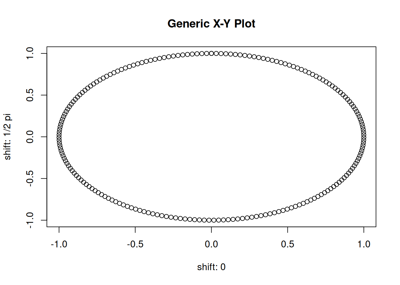
This is nothing else than plotting plot(m[, 1], m[, 2]).
Matrix plot
matplot() is plotting data columnwise. Each column will get a different
color and line type (or symbol if type = "p"; default) starting with color/line type 1
for the first column (black), 2 for the second (red) and so on.
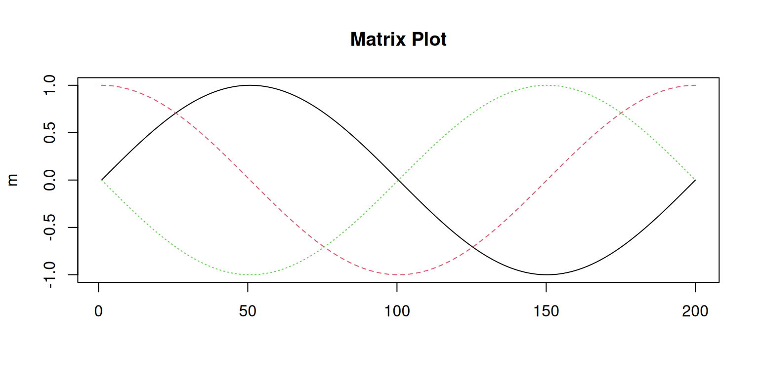
By default, the data are plotted against the row index. Thus, the x-axis shows
values between 1 and 200. To use custom values on the x-axis where we
want the data to be plotted, matplot(x, m, ...) can be used where the first input argument (x)
is a numeric vector specifying the values along the x-axis (in this example seq(0, 2 * pi, length.out = 200) from above),
the second input argument (m) the matrix containing the values plotted on the y-axis.
# Same matrix; specify additional values
# along the x-axis.
matplot(x, m,
        type = "l",
        xlab = NA,
        main = "Customized Matrix Plot")
# Display legend
legend("bottomleft", legend = colnames(m), col = 1:3, lty = 1:3)
# Adding custom second axis
axis(side = 1,
     at = c(0, pi, 2 * pi),
     line = 2,
     lwd = 0,
     c(expression(0), expression(pi), expression(2 * pi)),
     col = "steelblue")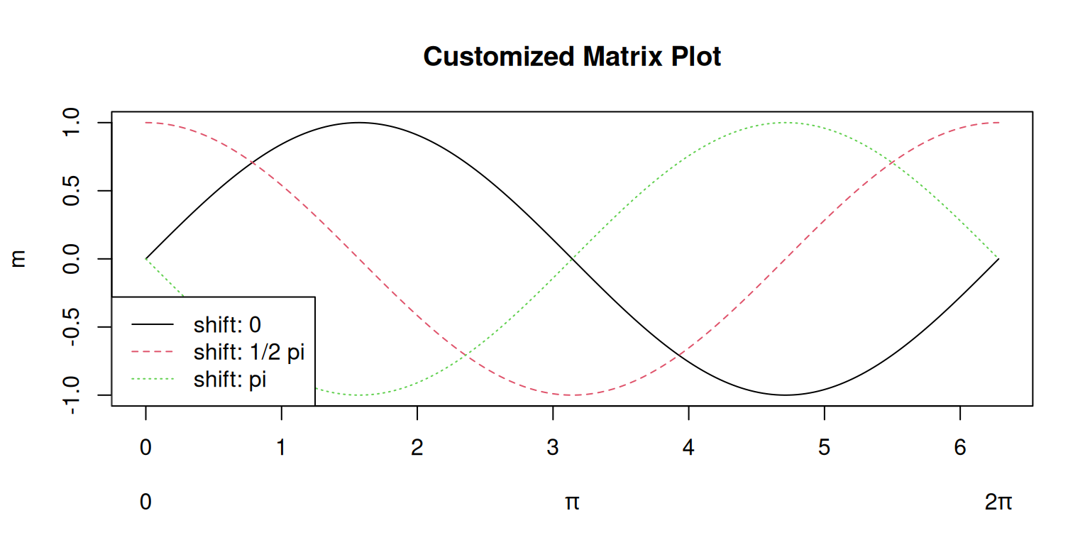
Image plot
For two dimensional data the image() function can be used. For demonstration
we use a data set called volcano – an elevation map of a volcano in New Zealand.
This is one of the data sets shipped with base R and can be loaded using:
This will create an object called volcano which simply is a numeric matrix.
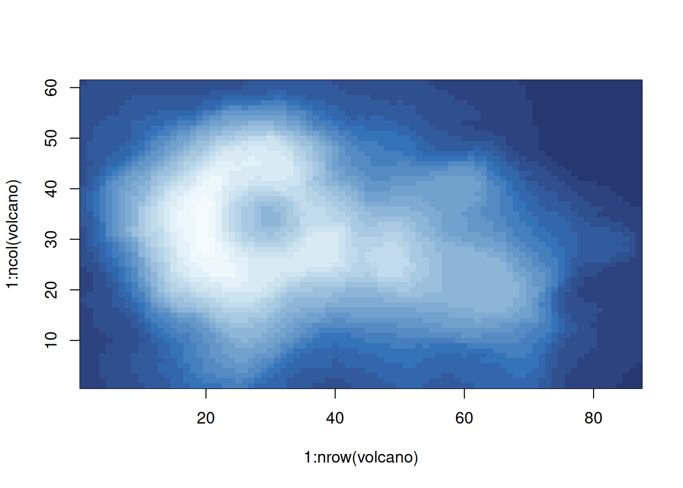
## [1] "matrix" "array"## [1] 87 61image() creates one rectangle (a ‘pixel’) for each element in the matrix.
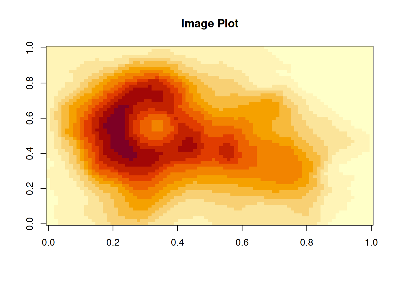
By default, both axis are set to \(0 - 1\) which can be changed if needed.
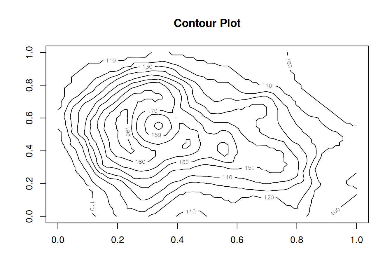
Contour plots
A contour plot (or level plot) works similar as the image() plot but plotting
a series of contours (or iso lines; lines of a constant value) as you may know
from e.g., hiking maps.
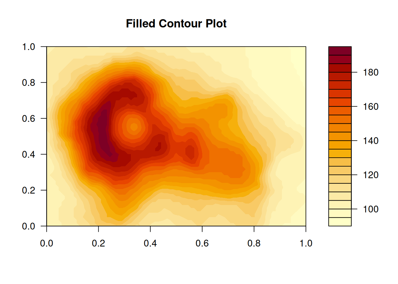
Filled contour plot
The filled contour plot does the same as contour() but fills the area between two
contours (two levels) instead of drawing them as lines. The result looks similar to what
the output of image(), but is smoother as the levels (contours) are interpolated
across the area.
All functions come with a series of options to customize the plots. For details
check out the corresponding help pages: ?matplot, ?image, ?contour, or ?filled.contour.