Chapter 8 Loops
In the previous chapter we were looking at conditional execution, this time we are looking at repetitive execution, often simply called loops. As if-statements, loops are not functions, but control statements.
Remember the flowchart from the previous chapter? The bottom right corner shows a ‘procrastination loop’: As long as you have more than 12 hours to submit your homework (condition), watch some TV, then check mails, …, check the time (action), and check again if you still have more than 12 hours to finish your homework (evaluate condition again). This is repeated until the condition is fulfilled.
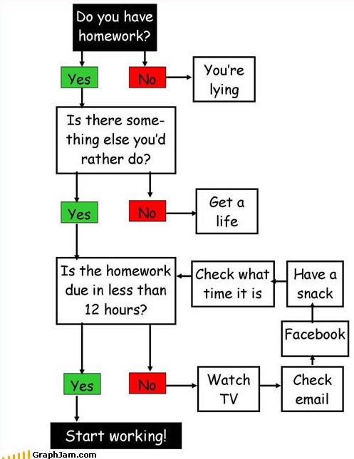
Figure 8.1: Source: GraphJam.com (offline).
8.1 for loops
The simplest and most frequently used type of loops is the for loop. For
loops in R always iterate over a sequence (a vector), where the length of the
vector defines how often the action inside the loop is executed.
Basic usage: for (<value> in <values>) { <action> }
<value>: Current loop variable.<values>: Set over which the variable iterates. Typically an atomic vector but can also be a list.<action>: Executed for each<value>in<values>.{...}: As for functions or if-statements – necessary when multiple commands are executed, optional for a single command.
A typical use is to loop over an integer sequence \(i = 1, 2, 3, ..., n\). The corresponding for-loop looks as follows:
- In R:
for (i in 1:n) { ... }. - In some other languages:
for (i = 1; i <= n; i ++) { ... }. This or a similar construct does not exist in R.
To see how this works, the two code chunks below show two examples where
we once loop over an integer sequence 1:3 (1:3)
and a character vector c("Reto", "Ben", "Lea").
## [1] 1
## [1] 2
## [1] 3## [1] "Reto"
## [1] "Ben"
## [1] "Lea"Explanation: R loops over the entire vector, element by element.
- For the first iteration, the first element of the vector is assigned to the
loop variable
i. - After reaching the end, the loop continues by assigning the second value to
the loop variable
i(second iteration). - This is done until there are no elements left – in this case three iterations. This ends the loop.
The loop variable (i) is a normal R object and can be used inside the loop
like any other object, here simply forwarded to the function print().
Instead of creating the vectors ‘on the fly’, we can also use existing vectors. Let us assign the vectors we are looping over before calling the loop:
## [1] 1
## [1] 2
## [1] 3
# Character vector
participants <- c("Reto", "Ben", "Lea")
# Use vector 'participants' for the loop.
for (name in participants) {
print(name)
}## [1] "Reto"
## [1] "Ben"
## [1] "Lea"As you can see we can also change the name for the loop variable (name).
i (as well as j, k, …) are indices often used in math, we’ll come
back to this in the section Nested for loops.
Backward loops
There are no special statements to loop backwards. Instead, we
simply reverse the values in the vector we use. 3:1 creates the reverse sequence of 1:3,
or we can make use of the function rev() to revert any vector.
## [1] 8 9 10 11## [1] 11 10 9 8Examples:
## [1] 3
## [1] 2
## [1] 1## [1] "Lea"
## [1] "Ben"
## [1] "Reto"Loops and subsetting
Loops are often used in combination with subsetting. We have a
named vector info with two elements:
and would like to loop over all elements (1:2) of the vector. Instead of only
printing 1 and 2 we use subetting by index to extract the values from the
vector above.
## [1] "Element 1 contains Innsbruck"
## [1] "Element 2 contains Austria"
Instead of looping over the indices (1:2) we could also loop over the
names of the vector (using names() to extract the character vector) and
use subsetting by name.
## [1] "Element name contains Innsbruck"
## [1] "Element country contains Austria"
Typical errors
A typical error is that the index (the sequence we loop over) is not properly constructed. The classical mistakes made (you may run into it as well):
- Wrong hard-coded range:
1:3instead of1:2. This would cause problems as our vector (info) only have 2, not 3 elements. - Incomplete range:
2instead of1:2.2is not a sequence, but a vector which contains one single value2. Thus, the loop would only loop overc(2).
Note: We should avoid hard-coding indices in general. Hard-coding means
that we explicitly write numbers like 1:2 into the code. What if the data
set or vector changes its length? Our loop may no longer work properly.
Better: Instead of using hard-coded sequences, we make use of length()
to check the length of the vector and use 1:length(info) to create the
vector. In case the length of info changes, the number of iterations
will change as well.
## [1] "Element 1 is Innsbruck"
## [1] "Element 2 is Austria"Zero-length: Be aware of zero-length vectors! Imagine that our vector
info may at some point become an empty vector (0 elements). In this
case 1:length(info) creates a sequence 1:0 which is c(1, 0) – and will cause problems.
The example below demonstrates this, but uses a new vector x instead of info (not to
lose our object info as we may need it again).
## [1] 0## [1] 1 0## [1] "Element 1: NA"
## [1] "Element 0: "This loop now iterates over i = 1 and i = 0. The vector x itself
has zero elements, and we get an NA for x[1] and an empty element for x[0].
Best solution: The most fail-safe solution is to use the
functions seq_len() or seq_along() which we have already seen
quickly in Creating vectors: Numeric sequences.
## [1] 1 2## [1] 1 2This also works with empty vectors as the two functions will return an empty sequence as well.
## [1] 0## integer(0)## integer(0)When used in a loop, an empty index vector means “don’t do even a single iteration”,
or in other words, the actions in the loop are never executed. The same example as
above but using seq_along(x) instead of 1:length(x):
No output as there are no iterations (length(seq_along(x)) == 0).
Nested for loops
For loops can also be nested. This is not only good to understand subsetting, but is also used relatively frequently. As nested conditions (see Conditional execution: Nested conditions), nested for loops are two (or more) independent for-loops nested inside one another.
Example of a nested loop:
## [1] "i = 1 j = 1"
## [1] "i = 1 j = 2"
## [1] "i = 1 j = 3"
## [1] "i = 2 j = 1"
## [1] "i = 2 j = 2"
## [1] "i = 2 j = 3"
This happens in detail:
- Set
i = 1L(outer loop)- Set
j = 1L(inner loop),istays1L - Set
j = 2L(inner loop),istays1L - Set
j = 3L(inner loop),istays1L - Inner loop finishes, proceed with outer loop
- Set
- Increase
i = 2L(outer loop)- Set
j = 1L(inner loop),istays2L - Set
j = 2L(inner loop),istays2L - Set
j = 3L(inner loop),istays2L - Inner loop finishes, proceed with outer loop
- Set
- Outer loop finishes as well, job done.
Loops and matrices
By row index and column index
A typical example is to loop over all elements in a matrix with a row index i and
a column index j. Remember the illustration from chapter Matrices?
Here is the same representation again for a slightly smaller matrix of dimension \(2 \times 3\):
\[ x = \underbrace{\left(\begin{array}{cc} x_{11} & x_{12} & x_{13} \\ x_{21} & x_{22} & x_{23} \\ \end{array}\right)}_{\text{Mathematical}\\\text{representation}} = \underbrace{\left(\begin{array}{cccc} \text{x}[{\color{blue}{1}}, {\color{red}{1}}] & \text{x}[{\color{blue}{1}}, {\color{red}{2}}] & {\text{x}[\color{blue}{1}}, {\color{red}{3}}] \\ \text{x}[{\color{blue}{2}}, {\color{red}{1}}] & \text{x}[{\color{blue}{2}}, {\color{red}{2}}] & {\text{x}[\color{blue}{2}}, {\color{red}{3}}] \\ \end{array}\right)}_{\text{R-like}\\\text{representation}} \]
Each element in the matrix is defined by its row index (blue) and column index (red). In mathematics, the index \(i\) is often used for the row index, and \(j\) for the column index.
To access each element once, we need to loop over all possible combinations
of i in 1:2 and j in 1:3 which is exactly what the nested for-loop shown above does.
Let us do the same thing on an actual matrix and use subsetting by index
to access each element exactly once
(see Matrices: Subsetting matrices):
##      [,1] [,2] [,3]
## [1,]    9    3    5
## [2,]    0   17    2
# Loop
for (i in 1:2) {
for (j in 1:3) {
print(paste0("Element x[", i, ", ", j, "] is ", x[i, j]))
}
}## [1] "Element x[1, 1] is 9"
## [1] "Element x[1, 2] is 3"
## [1] "Element x[1, 3] is 5"
## [1] "Element x[2, 1] is 0"
## [1] "Element x[2, 2] is 17"
## [1] "Element x[2, 3] is 2"Note that it is crucial to not mix up the dimensions and/or indices. The following loop …
## [1] "Element x[1, 1] is 9"
## [1] "Element x[1, 2] is 3"
## [1] "Element x[2, 1] is 0"
## [1] "Element x[2, 2] is 17"
## Error in x[i, j]: subscript out of bounds… runs into an error (subscript out of bounds). The reason: I wrongly
specified i = 1:3 and j = 1:2. Thus, the loop tries to access x[3, 1] at
some point which does not exist
(see Matrices: Out-of-range indices).
Hard-coded index vectors: Again, hard-coding i = 1:2 and j = 1:3 works well for this example, but should be avoided
in situations where the dimension of the matrix may change. As shown in the previous section
we better make use of 1:ncol(x) and 1:nrow(x),
## [1] 1 2## [1] 1 2 3… or even seq_len(nrow(x)) and seq_len(ncol(x)) to avoid problems
if we have zero rows or zero columns
(yes, matrices with no rows or no columns can actually exist).
## [1] 1 2## [1] 1 2 3Let us create a matrix with no rows by subsetting ‘no row’, all columns. This is not something we create by purpose, but might happen if your subsetting goes wrong at some point.
# Create a matrix with no rows
x <- matrix(1:6, nrow = 2)
y <- x[vector("integer", 0), , drop = FALSE]
When looking at the dimension of our new object y we see that this matrix
has actually zero rows, but three columns. If we would use 1:nrow(y) in a
loop we would again loop over c(1, 0) which will definitively cause problems.
## [1] 0 3## [1] 1 0## integer(0)By name
Alternatively we can also loop over all elements using the row names and column
names if we have a named matrix. This works the very same as for named vectors,
except using rownames() and colnames().
# Create demo matrix
(x <- matrix(c(28, 35, 13, 13, 1.62, 1.53, 1.83, 1.71, 65, 59, 72, 83),
             nrow = 4, dimnames = list(c("Veronica", "Karl", "Miriam", "Peter"),
                                       c("Age", "Size", "Weight"))))
## Age Size Weight
## Veronica 28 1.62 65
## Karl 35 1.53 59
## Miriam 13 1.83 72
## Peter 13 1.71 83for (rname in rownames(x)) {
for (cname in colnames(x)) {
print(paste("The", cname, "of", rname, "is", x[rname, cname]))
}
}## [1] "The Age of Veronica is 28"
## [1] "The Size of Veronica is 1.62"
## [1] "The Weight of Veronica is 65"
## [1] "The Age of Karl is 35"
## [1] "The Size of Karl is 1.53"
## [1] "The Weight of Karl is 59"
## [1] "The Age of Miriam is 13"
## [1] "The Size of Miriam is 1.83"
## [1] "The Weight of Miriam is 72"
## [1] "The Age of Peter is 13"
## [1] "The Size of Peter is 1.71"
## [1] "The Weight of Peter is 83"A more applied example: We would like to get the average values for all three columns. This can be done with a single loop:
- Loop over all columns by name.
- Extract the current column.
- Calculate the average (arithmetic mean).
## [1] "Average Age is 22.25"
## [1] "Average Size is 1.6725"
## [1] "Average Weight is 69.75"
Loops and conditional execution
To create more dynamic loops we can also combine loops (not limited to for
loops) and additional if-statements. The code chunk below shows an example of
a loop with conditional execution. Before you execute the code: Can you
see what the outcome of this loop will be?
More seriously: This combination can be used to select certain elements from a pair of vectors. We have two vectors with the first name and last name of some people.
first_name <- c("Lea",     "Sabine", "Mario", "Lea", "Peter",   "Max")
last_name  <- c("Schmidt", "Gross",  "Super", "Kah", "Steiner", "Muster")
What we want to do is to find everyone called ‘Lea’ and print their first and last name. This can be done as follows:
# Looping over index/position:
for (i in seq_along(first_name)) {
    # Check if first_name[i] is Lea. If so, print.
    if (first_name[i] == "Lea") {
        print(paste("Found:", first_name[i], last_name[i]))
    }
}
## [1] "Found: Lea Schmidt"
## [1] "Found: Lea Kah"Use next and break
Additional control constructs exist which can be used in combination with loops.
next: Skip current loop iteration and continue with the next one.break: Break from the entire loop (stop loop and jump to the end).
Technically these constructs are reserved words (try next <- 3, break <- "xyz") and not functions, thus no round brackets (not next() or break()).
Conditional next:
Conditional break:
As shown, both are used the same way, it only differs what will happen. For demonstration, let us execute the loop three times with different conditions:
- The original one as shown above.
- Adding a conditional
nextafter the print. - Adding a conditional
breakafter the print.
# Re-declare the data set
first_name <- c("Lea",     "Sabine", "Mario", "Lea", "Peter",   "Max")
last_name  <- c("Schmidt", "Gross",  "Super", "Kah", "Steiner", "Muster")

# Conditional next
for (i in seq_along(first_name)) {
    if (first_name[i] == "Lea") {
        print(paste("Found:", first_name[i], last_name[i]))
    }
}
## [1] "Found: Lea Schmidt"
## [1] "Found: Lea Kah"# Conditional next
for (i in seq_along(first_name)) {
if (first_name[i] == "Lea") {
print(paste("Found:", first_name[i], last_name[i]))
next
}
}## [1] "Found: Lea Schmidt"
## [1] "Found: Lea Kah"# Conditional break
for (i in seq_along(first_name)) {
if (first_name[i] == "Lea") {
print(paste("Found:", first_name[i], last_name[i]))
break
}
}## [1] "Found: Lea Schmidt"All Leas vs. first Lea: As you can see, the output of the three loops is not identical. All loops start with iteration one and check if the first person is a Lea. If not, start iteration two. The difference is the procedure when a Lea is found.
- Version 1: Prints the entry, the rest of the ‘action’ is then executed (there is nothing in this example) and the next iteration is started.
- Version 2: Prints the entry, then calls
next.nextforces the loop to immediately start the next iteration; any action belownextwould be ignored in the iteration in which it is called. - Version 3: Prints the entry, then calls
break.breakforces the entire loop to end immediately. Thus, as soon as the first Lea is found, the loop stops (no further iterations) and we only get the first match.
Exercise 8.1 Small exercise/riddle: Try to solve the following one without using
a computer. What is the final value of x?
Solution.
## [1] 3The loop runs for eight iterations (i = 1, up to i = 10), there is no
break statement which would stop the loop early.
- We start with
x <- 1andi = 1. - As long as
i <= 8(1 - 8) the conditioni <= 8is true andnextis called. This forces the loop to immediately start the next iteration and ignorex <- x + 1during the current iteration. - Once we reach
i = 9we finally get tox <- x + 1and increasexby one. This happens only twice, fori = 9andi = 10.
Thus, the final result must be the initial value plus two, 1 + 2.
Exercise 8.2 Small exercise/riddle: Try to solve it without executing the code.
What is the result of y after the following short loop?
Solution.
## [1] 2The result is 2. The tricky part here is the definition of the loop index :).
We initialize y <- 1 and then loop over i in 0. 0 itself is a numeric
vector of length 1! Thus the loop runs once, wherefore we once call y <- y + 1 and end up with 2.
## [1] "Element 1 of x is 0"## [1] 1Exercise 8.3 Small exercise/riddle: Another short for loop to activate
some brain cells. Which value takes z after running the following code?
Try to solve without executing the code again.
Solution.
## [1] 4The final result is 4. next here has basically no effect, but will be
included below for the sake of completeness.
- Initialize
z <- 0(zis 0). - Iteration 1 (
i = 1):z <- z + 1(zgets 1.0).- Condition
FALSE, don’t call break. z <- z + 0.5(zgets 1.5).- Call
next: before actually reaching}, start next iteration.
- Iteration 2 (
i = 2):z <- z + 1(zgets 2.5).- Condition
FALSE, don’t call break. z <- z + 0.5(zgets 3.0).- Call
next: before actually reaching}, start next iteration.
- Iteration 3 (
i = 3):z <- z + 1(zgets 4.0).i > 2isTRUE, callbreak. Immediately stops the execution of the loop.
The loop would have been run up to iteration i = 5, but this is never reached
as the break command is called early.
8.2 while loops
The second type of loop is while. In contrast to a for-loop which runs
for a fixed number of iterations, a while-loop runs while a condition is true.
Basic usage: while (<condition>) { <action> }.
<condition>: Logical condition, has to beFALSEorTRUE.<action>: Executed as long as the<condition>isTRUE.{...}: Necessary for multiple commands, optional for single ones.
Beware of infinite loops! A simple example for an infinite loop is the following simple while-loop.
This will run forever, as we start with x <- 1, wherefore x > 0 is TRUE,
and then increase the object by one in each iteration. All this loop does is
to basically count to infinity and will ‘never’ stop.
Figure 8.2: Infinite loop. Source: XKCD.
Useful while loop example
The following shows an example where a while-loop is useful in practice.
We want to print all numbers x in \(1, 2, ..., \infty\) as
long as x^2 is lower than 20, starting with x <- 0.
# Start with 0
x <- 0
# Loop until condition is FALSE
while (x^2 < 20) {
  print(x)      # Print x
  x <- x + 1    # Increase x by 1
}
## [1] 0
## [1] 1
## [1] 2
## [1] 3
## [1] 4xis 0, \(0^2 = 0\) \(\rightarrow\)x^2 < 20isTRUE; Increase x, continue.xis 1, \(1^2 = 1\) \(\rightarrow\)x^2 < 20isTRUE; Increase x, continue.xis 2, \(2^2 = 4\) \(\rightarrow\)x^2 < 20isTRUE; Increase x, continue.xis 3, \(3^2 = 9\) \(\rightarrow\)x^2 < 20isTRUE; Increase x, continue.xis 4, \(4^2 = 16\) \(\rightarrow\)x^2 < 20isTRUE; Increase x, continue.xis 5, \(5^2 = 25\);x^2 < 20is nowFALSE, wherefore the loop stops.
8.3 repeat loops
The last one is a repeat-loop. In contrast to the other two the repeat loop
runs forever – until we explicitly stop it by calling break.
Basic usage: repeat { <action> }.
<action>: Executed until thebreakstatement is called. Thus, don’t forget to includebreak.{...}: Necessary for multiple commands, optional for single ones.
Remarks:
- More rarely used compared to
forandwhileloops. - Not necessary for any task in this course!
- (But super simple to write).
Example: We could use a repeat loop to solve the same task as shown above
where we would like to get all numbers \(x \in [0, 1, ..., \infty]\) where \(x^2 < 20\)
like this:
# Initialization
x <- 0
# Repeat loop
repeat {
    if (x^2 > 20) break     # Break condition (important)
    print(x)                # print(x)
    x <- x + 1              # Increase x by 1
}
## [1] 0
## [1] 1
## [1] 2
## [1] 3
## [1] 48.4 Interim results
Sometimes one needs to use interim results (values/results which differ in each iteration) for recursive computations or to get more insights and further process the data.
To be able to do so, we need to store the interim results calculated in each of the iterations such that we can access them after the loop has finished.
There are two strategies to do so:
- Fixed: If we know how many elements we need to store (how many iterations we have in our loop): Pre-specify an object of suitable dimension before the loop is called.
- Dynamic: If we don’t know the number of iterations the dimension of the object can dynamically be extended. Much less efficient than the first version.
Fixed
In this example we write a loop which iterates 6 times. In each iteration the result from the previous iteration is taken and multiplied (recursive computation). Below, the same problem is defined once using mathematical notation, and once using pseudo-code.
Example: Mathematical definition.
- Initialize \(x_1 = 1\).
- Recursively set \(x_i = 1.5 \cdot x_{i - 1}\) for \(i = 2, ..., N\).
- In this example, \(N = 7\) (fixed number of iterations).
Explanation: Same problem explained in a different way (pseudo-code).
- Initialize
N <- 7(maximum number of iterations; fixed length). - Initialize a new (empty) numeric vector
xof length 7 (to store interim results). - Set
x[1](\(x_1\)) to 1 (starting value). - Write for-loop which iterates over
i = 2:N. In each iteration:- Take
x[i - 1]from the previous iteration (\(x_{i - 1}\)), - multiply
x[i - 1]by1.5, and - store the new value on
x[i](current iteration).
- Take
The code for this looks as follows:
## [1] 0 0 0 0 0 0 0## [1] 1# The loop
for (i in 2:N) {
# Do the calculation. Take 'x' from the previous (i-1)
# iteration, multiply, store on x[i] (current iteration).
x[i] <- 1.5 * x[i - 1]
}
print(x)## [1] 1.00000 1.50000 2.25000 3.37500 5.06250 7.59375 11.39062The ‘trick’ here is that the relative position changes trough the
iterations. We have learned how to subset objects by index. The index
we use is the absolute position of an element in the object.
The graphical representation below shows the vector x with a length of 7
as used in the example.
Absolute index: Here x[1:7], never changes. The leftmost element is
always x[1].

Relative index: In contrast to the absolute index, the relative
index changes. The images below show the relative indices, relative
to i (top down: i = 1, i = 2, i = 3).


Back to the example: In the beginning we create a new empty vector and set
x[1] (absolute index) to 1. Thus, our vector looks as follows after
initialization:

After initialization we start the loop. We are looping over
i in 2:N and use relative indices to access specific elements of the
vector x relative to the current loop index i.
The first iteration sets i = 2. Thus, x[i] <- 1.5 * x[i - 1] (relative)
implies nothing else than x[2] <- 1.5 * x[1] (absolute).

The very same happens for i = 3, implying x[3] <- 1.5 * x[2] …

… and all following iterations up to i = 7 (implying x[7] <- 1.5 * x[6]),
where the relative indices
look like this:


Dynamic
When we don’t know how much elements we need to store, we can dynamically extend the object we use to store our interim results. Depending on your object there are different functions to do so.
| Function | Description |
|---|---|
c() |
Combine vector elements (append elements). |
append() |
Add elements to a vector (similar to c() but slower). |
rbind() |
Add rows to a matrix. |
cbind() |
Add columns to a matrix. |
Exercise: Let us reuse the exercise from the previous section. This time, however, we will not have a fixed number of iterations (\(N = 7\)), instead we would like to continue with our recursive calculation until we exceed 10.
- Initialize \(x_1 = 1\).
- Recursively set \(x_i = 1.5 \cdot x_{i - 1}\) for \(i = {2, ..., N}\).
Repeat this step until
x[i] > 10(stop if this condition is met).
This is a classical example for a while-loop or a repeat-loop, both
are possible. Let us start with a while-loop. To be able
to easily use the relative indices needed, we define an additional
object i to count in which iteration we are at the moment.
Using a while-loop
x <- c(1)        # The initial value
i <- 1           # Initialize i = 1

# The loop. The while condition is 'x[i] < 10';
# Stops as soon as this condition is no longer TRUE.
while(x[i] < 10) {
    # Calculate new interim result
    # Combine existing vector x with new result
    x <- c(x, 1.5 * x[i])

    # Increase iteration counter after calculation.
    # Could be done before (changes relative index position!).
    i <- i + 1
}
x
## [1] 1.00000 1.50000 2.25000 3.37500 5.06250 7.59375 11.39062How many iterations did it take? We can either check our variable i or the length
of our vector x. Careful: the first element (x[1]) was the initial/starting
value and not iteration one, thus, we need to take that into account (-1).
## [1] 6## [1] 6Different while-loop
We could write the loop differently without using a loop counter. Instead, we
use tail(x, n = 1) to always get the last element of x.
x <- c(1)        # The initial value
# Loop
while (tail(x, n = 1) < 10) {
    x <- c(x, 1.5 * tail(x, n = 1))
}
x
## [1] 1.00000 1.50000 2.25000 3.37500 5.06250 7.59375 11.39062## [1] 7Repeat-loop
Instead of using a while loop we could use a repeat-loop and
use the condition to call the break statement as soon as
our newest value in x exceeds 10. Using an iteration counter is
not necessary but is, again, a possible solution to this problem.
# With iteration counter
x <- c(1)
i <- 1
repeat {
    # Break condition before calculation
    if (x[i] > 10) break
    # Calculation
    x <- c(x, 1.5 * x[i])
    # Increase loop counter
    i <- i + 1
}
x
## [1] 1.00000 1.50000 2.25000 3.37500 5.06250 7.59375 11.39062# Without iteration counter (make use of tail())
x <- c(1)
repeat {
# Calculation
x <- c(x, 1.5 * tail(x, n = 1))
# Break condition after calculation
if (tail(x, n = 1) > 10) break
}
x## [1] 1.00000 1.50000 2.25000 3.37500 5.06250 7.59375 11.39062As you can see, there are often very different approaches to solve the same problem. The ‘best’ or most optimal solution often depends on the task itself.
Efficiency
It was mentioned that the approach using a predefined object with fixed dimension is faster than the one using dynamic extension of the resulting object.
There are ways to test this. One example is the microbenchmark package. This goes beyond the scope of this course – you don’t need to know this. But it might be good to know that this exists. Especially when working on programs/software in the real world the execution time is often a crucial element of a project.
Package required: We will use an additional R package called microbenchmark. This is not part of base R and must be installed before we can use it. The package can be installed (as all other packages on CRAN) by calling:
install.packages("microbenchmark")
This should download and install the package into your personal ‘package library’. A package is like an additonal module which adds additional functionality to R.
Once installed, we have to load the package from the library using the command
library("microbenchmark") before we are able to use the new features/functions/tools.
We will compare two super simple loops which create an integer sequence.
- For-loop: iterates over
i = 1:1000; Storesiinto fixed-length vectorx. - While-loop: iterates until
i > 1000(1000 times); Extends vectorxdynamically to storei.
# Loading the library
library("microbenchmark")
microbenchmark("for-loop (fixed)" = {
    # For-loop
    x <- vector("integer", 1000)
    for (i in 1:1000) { x[i] <- i }
  }, "while-loop (dynamic)" = {
    x <- c()
    i <- 1
    while (i <= 1000) { x <- c(x, i); i <- i + 1 }
  }, check = "equal", times = 100L, unit = "ms")
## Unit: milliseconds
## expr min lq mean median uq max
## for-loop (fixed) 1.223572 1.487912 1.555298 1.526471 1.626333 2.250462
## while-loop (dynamic) 2.321333 2.782860 3.231141 2.947377 3.133133 7.575593
## neval cld
## 100 a
## 100 bmicrobenchmark() executes both versions 100 times (times = 100)
and returns the time required to execute the two code chunks.
On average, the for-loop with fixed assignment is about twice as fast as the while loop. The main reason is that the while-loop has to extend the vector every time, over and over again. The absolute difference here is in the milliseconds. However, when you have a larger script – making it twice as fast as before – can save enormous amounts of time (and nerves).
Note: times vary from computer to computer, and time to time.
For a real problem one might also increase the times argument to
a larger number to get more stable/reliable results.
8.5 Loop replacements
Instead of the three basic repetitive control structures (for, while, and
repeat) R comes with a series of functions which can be used as
replacements. These ‘loop replacements’ are real functions (no longer control
statements). The following exist:
| Function | Description |
|---|---|
apply() |
Apply a function over margins of an array (e.g., over rows or columns of a matrix). |
lapply() |
Apply a function over a vector or list, returns a list. |
sapply() |
Like lapply() but tries to simplify the result to a vector or matrix. |
vapply() |
Like sapply() but with pre-specified return value. |
tapply() |
Apply a function over a ragged array (e.g., within groups) and return a table. |
Remarks:
- Often easier and/or more compact to write than explicit loops.
- In early versions of R also more efficient than loops – now comparable.
- In this chapter we will solely focus on
apply(). - Other functions will be discussed later along with lists and data frames.
Usage from the manual:
Usage:
     apply(X, MARGIN, FUN, ...)

Arguments:
       X: an array, including a matrix.
  MARGIN: a vector giving the subscripts which the function will be
          applied over.  E.g., for a matrix ‘1’ indicates rows, ‘2’
          indicates columns, ‘c(1, 2)’ indicates rows and columns.
     FUN: the function to be applied.
     ...: optional arguments to ‘FUN’.
Over columns
Example: Let us use a \(4 \times 5\) matrix with random values.
##               A          B          C           D           E
## [1,] -0.6264538  0.3295078  0.5757814 -0.62124058 -0.01619026
## [2,]  0.1836433 -0.8204684 -0.3053884 -2.21469989  0.94383621
## [3,] -0.8356286  0.4874291  1.5117812  1.12493092  0.82122120
## [4,]  1.5952808  0.7383247  0.3898432 -0.04493361  0.59390132
For each column of the matrix we would like to calculate the means, standard deviation and count all positive elements.
To calculate the mean over all columns, we need to call:
##           A           B           C           D           E
##  0.07921043  0.18369829  0.54300434 -0.43898579  0.58569212
The 2 (MARGIN = 2) indicates that we would like to apply the function
column-by-column. mean (FUN = mean) is the function to be applied.
As we have used a named matrix, we will get a named vector as a result.
The very same can be used to calculate the standard deviation.
##         A         B         C         D         E
## 1.1021597 0.6902835 0.7489618 1.3889432 0.4266423
However, there is no function which counts the ‘number of positive values’.
We have to write a custom function first, which will be called npos (number of positives).
Once defined, we can use our custom function in combination with apply().
## A B C D E
## 2 3 3 1 3
We can also use more complex functions with more than one input argument.
The following function can return both, the number of positive elements (if pos = TRUE; default), or the number of negative elements (if pos = FALSE).
## [1] 2## [1] 1When calling apply() we can provide additional arguments to the function
we apply by simply adding them (see ... argument).
## A B C D E
## 2 3 3 1 3## A B C D E
## 2 3 3 1 3## A B C D E
## 2 1 1 3 1Over rows
Analogously we can apply a function over the rows by simply changing
MARGIN = 2 to MARGIN = 1. As our matrix has no row names, the result
is an unnamed vector of the same length as nrow(x).
## [1] 2 2 4 4Over elements
If MARGIN = c(1, 2) we would like to keep both dimensions. In this
case the function is applied element-by-element.
##      A B C D E
## [1,] 0 1 1 0 0
## [2,] 1 0 0 0 1
## [3,] 0 1 1 1 1
## [4,] 1 1 1 0 1
This is getting very useful when you have multi-dimensional arrays (arrays with 3 or more dimensions) and you would like to calculate things over specific dimensions.
8.6 Summary
Different types of loops: Quick repetition of the differences between the three types of loops.
forloops: Loop over a vector (sequence); Repeat<action>for each element in the vector.whileloops: Repeat<action>as long as a logical expression isTRUE(e.g., until the expression evaluates toFALSE).repeatloops: Repeatforever – until a break(stop) is explicitly called.
Control-flow overview: The table below shows the commands (functions and statements) we have learned in this and the previous chapters used for flow control in R.
| Command | Description |
|---|---|
if and else |
Conditional execution in different variants. |
ifelse() |
Vectorized if. |
for |
Loop over a fixed number of items (a sequence). |
while |
Loop while a condition is TRUE |
repeat |
Infinite loop (until break stops execution). |
break |
Stop/break execution of a loop. |
next |
Skip iteration, continue loop. |
return |
Exit a function (returns result). |
In additon, a series of loop replacements exist. These are functions (not control statements)
and can be very handy for many tasks. We have been looking at apply() in this chapter,
but will come back to some more when talking about lists and data frames.