Chapter 10 Data Frames

10.1 Data frame introduction

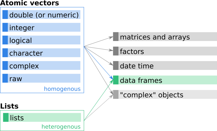
Figure 10.1: Data frames – a combination of lists and (most often) atomic vectors.

We can now combine our knowledge about lists and vectors to create a new object class, the so called data frame. Data frames are structured rectangular objects similar to matrices, but more flexible and constructed differently.

Reminder: So far we have only learned to use matrices to represent rectangular data and learned about the following properties.

• Matrices are vectors with an additional dimension attribute for rows and columns.
• As based on vectors, they must be homogeneous (numeric, character, …).
• An alternative object is needed for empirical data which typically contain heterogeneous columns.

Data frame: Most commonly used data type to represent rectangular data in R.

• Data frames are always two-dimensional objects.
• Columns of a data frame correspond to variables, rows to observations (different jargon).
• Look like a matrix and offer similar subsetting methods, but are not matrices.
• Internally, a data frame is a list with a series of objects of the same length.
• The list-elements (variables) are most often vectors of potentially different types, however, more complex objects such as lists or matrices (for specific variables) are possible.
• Variables (columns) are always named, the names are no longer optional.
• Observations (rows) also always have names, by default they are set to "1", "2", … but can be changed.

As mentioned, data frames look like matrices but are based on a list. This allows for a higher degree of flexibility than matrices as it now allows to store different types of data into different columns/variables, e.g., characters in the first column, integers in the second, and logical in the third.

10.2 Creating data frames

Not surprisingly, data frames are constructed using the function data.frame(). The function works very similar to list() with some additional options. Let us have a look at the usage from the manual (see ?data.frame).

Constructor function:

data.frame(..., row.names = NULL, check.rows = FALSE,
           check.names = TRUE, fix.empty.names = TRUE,
           stringsAsFactors = default.stringsAsFactors())

Important arguments:

• ...: value or tag = value. Component names are created based on the tag (if present) or the deparsed argument itself.
• stringsAsFactors: logical: should character vectors be converted to factors? Default changed to FALSE in R 4.0.0.

The second argument is mentioned here as the default changed with R version 4.0.0. Try to keep that in mind as it get important when using existing (older) R scripts or you work on a computer/server with an old R installation. For now we will ignore this as we will talk about ‘factors’ in the next chapters.

Basic usage: Let us create a simple demo data frame with two variables. The first one is an integer sequence of length \(3\), the second a character vector of length \(3\) as well.

data.frame(1:3, c("a", "b", "c"))

##   X1.3 c..a....b....c..
## 1    1                a
## 2    2                b
## 3    3                c

As we have not named our variables R tries to guess a name. Well, not very useful. What if we pre-specify the two vectors and call them x and y?

x <- 1:3
y <- c("a", "b", "c")
data.frame(x, y)

##   x y
## 1 1 a
## 2 2 b
## 3 3 c

Alternatively we can create a data frame with names by using a series of key = value arguments.

(df <- data.frame(age = c(35, 21, 12), height = c(1.72, 1.65, 1.39)))

##   age height
## 1  35   1.72
## 2  21   1.65
## 3  12   1.39

Heterogeneous data: The big advantage is that we can now create heterogeneous rectangular objects. The following example shows a data frame with four variables, all based on vectors of different types.

(df <- data.frame(
            name = c("Petra", "Jochen", "Alexander"),     # character
            age = c(35L, 21L, 12L),                       # integer
            height = c(1.72, 1.65, 1.39),                 # numeric
            austrian = c(FALSE, TRUE, TRUE),              # logical
            stringsAsFactors = FALSE                      # default
))

##        name age height austrian
## 1     Petra  35   1.72    FALSE
## 2    Jochen  21   1.65     TRUE
## 3 Alexander  12   1.39     TRUE

Let us now investigate the new object, first using the str() function.

str(df)

## 'data.frame':    3 obs. of  4 variables:
##  $ name    : chr  "Petra" "Jochen" "Alexander"
##  $ age     : int  35 21 12
##  $ height  : num  1.72 1.65 1.39
##  $ austrian: logi  FALSE TRUE TRUE

The output looks similar to the one for a list with a few important differences. The first line tells us that we are dealing with a data.frame with \(3\) observations (obs.) and \(4\) variables. Once more: ‘observations’ correspond to rows, variables to columns.

All other lines show the definition of the different variables. As a data frame is based on a list, the following lines show the different variables (each of which is an element in the underlying list). Thus, we can again see $ <name> followed by a brief description of the object stored inside, including the type (chr = character, int = integer, num = numeric, logi = logical) and the first few elements.

10.3 Data frame attributes

As all other objects data frames always have a type which is "list" and a length. Besides these properties, data frames always have at least the following three attributes:

• Class: Data frames are of class "data.frame".
• Dimension: 2-dimensional rectangular objects; always have a dimension attribute.
• Names: Data frames must always be named, no longer optional (as for matrices).

Let us look at the object df defined above and what class and type it comes with.

head(df, n = 1) # first observations (row)

##    name age height austrian
## 1 Petra  35   1.72    FALSE

class(df)       # Class is data.frame

## [1] "data.frame"

typeof(df)      # The underlying type is a list (based on a list)

## [1] "list"

The class is data.frame while the type is list, like matrices which are of class matrix, array, but the type is always one of the atomic types (double, integer, …). Again, a function exists to check if a given object is a data frame:

c("is.data.frame" = is.data.frame(df),
  "is.list"       = is.list(df),
  "is.matrix"     = is.matrix(df),
  "is.atomic"     = is.atomic(df))

## is.data.frame       is.list     is.matrix     is.atomic 
##          TRUE          TRUE         FALSE         FALSE

Note that is.data.frame() and is.list() both return TRUE! However, as shown a data frame is not a matrix, and also not atomic as based on a generic vector (list; see Lists).

The length of a data frame is the length of its underlying list, which is the same as the second dimension (or number of variables/columns). The first dimension (number of rows) tells us how many observations the data frame contains.

length(df)      # Length of underlying list

## [1] 4

dim(df)         # Like for matrices

## [1] 3 4

nrow(df)

## [1] 3

ncol(df)

## [1] 4

As data frames always have names, let us have a look what the three functions names(), colnames(), and rownames() return.

names(df)

## [1] "name"     "age"      "height"   "austrian"

colnames(df)

## [1] "name"     "age"      "height"   "austrian"

rownames(df)

## [1] "1" "2" "3"

names() and colnames() do the very same and return the names of the variables. When working with data frames one typically uses names() (not colnames()). In addition we can see that R automatically assigned the default row names "1", "2", and "3" as we have not specified anything different. As always: the return of these functions are character vectors!

10.4 Subsetting data frames

Subsetting combines the two worlds of lists and matrices. We can basically use all the subsetting techniques learned in the previous chapters. In addition we can use a function called subset() which becomes very handy when working with data frames.

Matrix/list-like

Some examples based on the following object:

(df <- data.frame(
            name = c("Petra", "Jochen", "Alexander"),     # character
            age = c(35L, 21L, 12L),                       # integer
            height = c(1.72, 1.65, 1.39),                 # numeric
            austrian = c(FALSE, TRUE, TRUE),              # logical
            stringsAsFactors = FALSE                      # default
))

##        name age height austrian
## 1     Petra  35   1.72    FALSE
## 2    Jochen  21   1.65     TRUE
## 3 Alexander  12   1.39     TRUE

List-style subsetting: The following subsetting commands all work (try it yourself, output not shown) on the data frame above.

Subsetting by positive or negative indices, single or double squared brackets to either get the content (element) or a subset (still a data frame but with less variables).

df[1]        # Returns sub-data-frame

##        name
## 1     Petra
## 2    Jochen
## 3 Alexander

df[-1]       # Sub-list (all except the first variable; negative index)

##   age height austrian
## 1  35   1.72    FALSE
## 2  21   1.65     TRUE
## 3  12   1.39     TRUE

df[[2]]      # Content of the second element

## [1] 35 21 12

Or use logical vectors for subsetting. This is most often only used with logical expressions.

df[c(TRUE, FALSE, TRUE, FALSE)]

##        name height
## 1     Petra   1.72
## 2    Jochen   1.65
## 3 Alexander   1.39

Subsetting by name using either squared brackets or the $ operator.

df["name"]   # Returns sub-data-frame

##        name
## 1     Petra
## 2    Jochen
## 3 Alexander

df$name      # Content of variable 'name'; preferred way

## [1] "Petra"     "Jochen"    "Alexander"

df[["name"]] # Content of variable 'name' as $name

## [1] "Petra"     "Jochen"    "Alexander"

And, last but not least, we could also use the recursive subsetting if needed. For example we could get the third list element (or variable/column) and extract the first element (or observation/row) from that.

df[[c(3, 1)]]     # Nested/recursive subsetting

## [1] 1.72

Matrix-style subsetting: In addition, we can use all matrix subsetting techniques to get specific elements (df[1, 3]), entire rows/observations (df[1, ]), or specific columns/variables (df[, 2]). This can be done using indices, names, or logical vectors (just as for matrices).

df[1, 3]      # Content of first observation (row), third variable (column)

## [1] 1.72

df[1, ]       # First observation (row); returns a data frame with one observation

##    name age height austrian
## 1 Petra  35   1.72    FALSE

df[, 1]       # First variable/column; returns the content

## [1] "Petra"     "Jochen"    "Alexander"

df[1, "name"] # Using names and indices

## [1] "Petra"

# By logical vectors
df[c(TRUE, FALSE, FALSE), c(TRUE, TRUE, FALSE, FALSE)]

##    name age
## 1 Petra  35

Mixed subsetting: We can of course combine subsetting techniques:

df$name[3]

## [1] "Alexander"

df[[2]][3]

## [1] 12

df[1, ]$name

## [1] "Petra"

df[df$height > 1.60, "austrian"]

## [1] FALSE  TRUE

The subset() function

The function subset() is another way to subset rows and columns of a data frame and is often more convenient to use.

Usage

## S3 method for class 'data.frame'
subset(x, subset, select, drop = FALSE, ...)

Important arguments

• x: object to be subsetted (not necessarily data frame).
• subset: logical expression indicating elements or rows to keep: missing values are taken as false.
• select: expression, indicating columns to select from a data frame.
• drop: passed on to ‘[’ indexing operator.

Example: Let us use the data frame from above.

(df <- data.frame(
            name = c("Petra", "Jochen", "Alexander"),     # character
            age = c(35L, 21L, 12L),                       # integer
            height = c(1.72, 1.65, 1.39),                 # numeric
            austrian = c(FALSE, TRUE, TRUE),              # logical
            stringsAsFactors = FALSE                      # default
))

##        name age height austrian
## 1     Petra  35   1.72    FALSE
## 2    Jochen  21   1.65     TRUE
## 3 Alexander  12   1.39     TRUE

Let us assume we are interested in all people which are 18 or older and we only want to have their name and height. The logical expression therefore would be df$age >= 18 and we could use this in combination with matrix-alike subsetting as follows:

# All rows where age >= 18, only columns c("name", "height")
df[df$age >= 18, c("name", "height")]

##     name height
## 1  Petra   1.72
## 2 Jochen   1.65

The same can be done using the subset() function.

subset(x = df, subset = age >= 18, select = c(name, height))

##     name height
## 1  Petra   1.72
## 2 Jochen   1.65

subset(df, age >= 18, c(name, height))

##     name height
## 1  Petra   1.72
## 2 Jochen   1.65

What the function does: it takes the first argument x and uses all variables/elements in this object to evaluate the additional arguments for subset and select (if specified). As shown, the variable names (age, name, height) are no longer in quotes. This works as R uses a technique called ‘non-standard evaluation’.

In the same way we could also get all non-Austrians in the data set. If we don’t define ‘select’ all variables/columns will be returned.

# The variable `austrian` is already a logical vector.
# `!austrian` negates the vector (turns every TRUE to FALSE and vice versa).
# Can be used to subset all non-austrians from the data frame `df`.
subset(df, !austrian)

##    name age height austrian
## 1 Petra  35   1.72    FALSE

The return of subset() will be a data frame if the first argument x is of class data frame – except if we select one row and set drop = TRUE. In this case we will only get a vector, in the example below a logical vector.

(x <- subset(df, age >= 18, austrian, drop = TRUE))

## [1] FALSE  TRUE

class(x)

## [1] "logical"

Graphical summary/recap

Short recap showing the differences and similarities between different ways of subsetting a data frame: Figure A and B below show subsetting without using the subset() method, while C summarizes the behaviour of the subset() method.

• A Subsetting observations (x[i, ]) or variables (x[j]):
  • Returns a data frame, subset of the original object x.
  • Allows to use indices (positive, negative, vectors), names, or logical vectors.
• B Subsetting (extracting) elements (values).
  • In case of x$var2, x[, j], or x[[j]] a vector is returned.
  • x[i, j] extracts a specific element (only if [i, j] defines one specific element!).
  • Allows to use indices (positive, negative, vectors), names, or logical vectors.
• C The subset() method allows to do everything from above.
  • Argument subset: subsetting observations.
  • Argument select: subsetting variables.
  • If drop = TRUE (default is FALSE) elements are returned, if possible.

10.5 Replacing/deleting/adding variables

Element-replacement works the same way as for lists. If we use subsetting and assign the value NULL, the variable will be deleted from the data frame.

df$name <- NULL
df

##   age height austrian
## 1  35   1.72    FALSE
## 2  21   1.65     TRUE
## 3  12   1.39     TRUE

We can also replace entire variables by assigning a new vector (take care of the length; recycling) on an existing variable, or adding new variables when using a new (not yet existing) variable name.

# Adds a completely new variable
df$nationality <- ifelse(df$austrian, "AT", NA)
# Replaces an existing colmn
df$height      <- as.integer(df$height * 100)
# Replace one element
df$age[2]      <- 102
# Print resulting data frame
df

##   age height austrian nationality
## 1  35    172    FALSE        <NA>
## 2 102    165     TRUE          AT
## 3  12    139     TRUE          AT

10.6 Coercing data frames

To some extent, we can coerce (convert) other R objects into data frames, or vice versa. However, this is only possible in certain situations.

Vector to data frame: A single vector yields a single-column data frame with one variable. The object name will be used as variable name.

name <- c("Jochen", "Martina")
as.data.frame(name)

##      name
## 1  Jochen
## 2 Martina

Matrix to data frame: Each column of the matrix will be converted into a variable. Row and column names will be preserved if specified, else R will add default values.

(mat <- matrix(1:6, nrow = 2, dimnames = list(c("Row 1", "Row 2"), LETTERS[1:3])))

##       A B C
## Row 1 1 3 5
## Row 2 2 4 6

(df <- as.data.frame(mat))

##       A B C
## Row 1 1 3 5
## Row 2 2 4 6

str(df)

## 'data.frame':    2 obs. of  3 variables:
##  $ A: int  1 2
##  $ B: int  3 4
##  $ C: int  5 6

This results in a homogeneous data frame (only contains integer variables). In this example we started with an integer matrix and converted the matrix into a data frame. This allows us to easily convert the data frame back into a matrix.

(mat2 <- as.matrix(df))

##       A B C
## Row 1 1 3 5
## Row 2 2 4 6

typeof(mat2)

## [1] "integer"

identical(mat, mat2)

## [1] TRUE

Going from mat \(\rightarrow\) df \(\rightarrow\) mat2 gets us the identical object as we have been started with. This does no longer work for heterogeneous data frames (shown next).

Heterogeneous data frames to matrix: Assume we have the following data frame again.

(df <- data.frame(
            name = c("Petra", "Jochen", "Alexander"),     # character
            age = c(35L, 21L, 12L),                       # integer
            height = c(1.72, 1.65, 1.39),                 # numeric
            austrian = c(FALSE, TRUE, TRUE),              # logical
            stringsAsFactors = FALSE                      # default
))

##        name age height austrian
## 1     Petra  35   1.72    FALSE
## 2    Jochen  21   1.65     TRUE
## 3 Alexander  12   1.39     TRUE

Can we convert this object into a matrix and back into a data frame without losing anything? The following line converts the object df into a matrix (as.matrix()) and directly back into a data frame (as.data.frame(...))).

# Coerce to matrix and back to data frame
(df2 <- as.data.frame(as.matrix(df)))

##        name age height austrian
## 1     Petra  35   1.72    FALSE
## 2    Jochen  21   1.65     TRUE
## 3 Alexander  12   1.39     TRUE

identical(df, df2)

## [1] FALSE

Well, seems it works. At least it does something. As we can see, df and df2 are no longer identical. Somethig important happened which will cause problems when working with this new df2 object as it is. For demonstration, let us calculate the arithmetic mean of the variable age.

mean(df2$age)

## Warning in mean.default(df2$age): argument is not numeric or logical: returning
## NA

## [1] NA

We get an NA and a warning, that our input was not numeric or logical. If we have a second look at the object df2 we can see that all our variables are now characters.

str(df2)

## 'data.frame':    3 obs. of  4 variables:
##  $ name    : chr  "Petra" "Jochen" "Alexander"
##  $ age     : chr  "35" "21" "12"
##  $ height  : chr  "1.72" "1.65" "1.39"
##  $ austrian: chr  "FALSE" "TRUE" "TRUE"

The reason is that when we convert the data frame to a matrix (as.matrix()) R has to convert the information in the data frame into a vector. As a vector (and thus matrices) can only contain data of one type, everything is converted into character in this case (see Vectors: Coercion). Take care of this!

List to data frame: As data frames are based on lists, we can always convert data frames to list, but also lists into a data frame. An example:

(df <- as.data.frame(list(x = c(1, 2, 3, 4), y = c("A", "B"))))

##   x y
## 1 1 A
## 2 2 B
## 3 3 A
## 4 4 B

Note: all variables of a data frame need to be of the same length! Thus, R is recycling the elements of the argument y such that the length matches the length of the longer argument x. When converting the data frame into a list, we will get the following:

as.list(df)

## $x
## [1] 1 2 3 4
## 
## $y
## [1] "A" "B" "A" "B"

10.7 Combining data frames

Data frames can also be combined. Let us assume we have the following three data frames containing the geographical position of some cities (df1, df2; name, latitude, longitude) and one data frame with the number of inhabitants for two cities (df3). We would like to combine them in one single object.

(df1 <- data.frame(name = c("Moskow", "Brasilia"),
                   lat  = c(55.8, -15.8),
                   long = c(37.6, -47.8)))

##       name   lat  long
## 1   Moskow  55.8  37.6
## 2 Brasilia -15.8 -47.8

(df2 <- data.frame(name = c("Innsbruck", "Graz"),
                   lat  = c(47.2, 47.4),
                   long = c(11.2, 15.3)))

##        name  lat long
## 1 Innsbruck 47.2 11.2
## 2      Graz 47.4 15.3

(df3 <- data.frame(name = c("Graz", "Innsbruck"),
                   inhabitants = c(294600, 132500)))

##        name inhabitants
## 1      Graz      294600
## 2 Innsbruck      132500

There are different functions to do so, however, they all have their difficulties. As for matrices, we can use cbind() and rbind() (with some limitations) or data.frame() to combine two data frames.

Row-binding: In case of df1 and df2 we could think of using row-binding as the two data frames do have the very same structure.

rbind(df1, df2)

##        name   lat  long
## 1    Moskow  55.8  37.6
## 2  Brasilia -15.8 -47.8
## 3 Innsbruck  47.2  11.2
## 4      Graz  47.4  15.3

This only works if the two data sets do have the very same variable names. Coercion will take place if the data type of some variables differ.

Column-binding: In the example of df2 and df3 we might combine the data frames side-by-side (column binding). The problem: R does not care about the content (we can see that we have a mismatch as the two data frames are in a different order; mixing information about Graz and Innsbruck).

cbind(df2, df3)

##        name  lat long      name inhabitants
## 1 Innsbruck 47.2 11.2      Graz      294600
## 2      Graz 47.4 15.3 Innsbruck      132500

Warning: elements will be recycled if the number of rows do not match. In addition we can see that we now have two variables called the very same ("name"). This is never a good idea and should be avoided!

Using data.frame(): As an alternative to cbind() we could use data.frame(). It takes care of duplicated variable names, however, has the same problems as cbind() regarding the mapping of the data.

data.frame(df2, df3)

##        name  lat long    name.1 inhabitants
## 1 Innsbruck 47.2 11.2      Graz      294600
## 2      Graz 47.4 15.3 Innsbruck      132500

Still not the best idea.

Merge: The best option for this case would be merge(). merge() merges two data frames. If we have the same variable in both data frames, this variable will be used to match the columns to be sure that we combine the correct values! In our case we have name in both data frames. Check the difference to before:

merge(df2, df3)

##        name  lat long inhabitants
## 1      Graz 47.4 15.3      294600
## 2 Innsbruck 47.2 11.2      132500

R auto-detects that we have one column with the same name. Given the value in "name" the observations of the two data frames will be brought in the same order – and then combined. The "name" variable is automatically used as the by argument (by which column the data should be merged). This can also be specified manually, e.g.,:

merge(df2, df3, by = "name")

##        name  lat long inhabitants
## 1      Graz 47.4 15.3      294600
## 2 Innsbruck 47.2 11.2      132500

In case the variables are named differently in the two data frames we could also define a by.x (variable name in the first data frame) and by.y (second data frame). The function merge() has a series of arguments, check ?merge for details.

Graphical summary/recap

A quick graphical summary of the different (correct and wrong) ways of combining data frames. We have three small data frames with two observations each. The first two (left) share the same variable names and contain geographical location of some cities. The last (right) shares the same values in one column (name) with the data frame bottom left, but contains different information.

Row binding: As the two data frames on the left have the same number of variables (columns) we can use rbind(df1, df2) to combine them. Warning: base R does not check what’s in the columns, it just binds them together!

If the two objects contain different number of variables, an error will be thrown (not possible).

Column binding: When having two objects with the same number of rows, we can call cbind(df2, df3). Again, cbind() does not care about what is in there, just combines them.

In this case this is a bad choice as we have duplicated information in two rows, and the observations/information is combined in a wrong way.

Merging: merge(df2, df3, by = "name") ‘column-binds’ information the information correctly. Compares the values in x$name and y$name and correctly combines the information.

10.8 Apply functions

In the chapter loops we discussed so called loop replacement functions (see Loop replacements) and have shown a function called apply() which can be used to apply a function to specific margins of a matrix. Beside apply() a series of additional *apply() functions exist used to replace more complicated loops.

Function	Return value
lapply()	Always returns a list.
sapply()	Tries to simplify the return to a vector or matrix.
vapply()	Tries to simplify to a pre-specified return value.

Usage: The usage for the three functions is very similar. Given the manual/help page:

lapply(X, FUN, ...)
sapply(X, FUN, ...)
vapply(X, FUN, FUN.VALUE, ...)

Important arguments:

• X: A vector (atomic or list) or an expression object. Other objects will be coerced by as.list().
• FUN: The function to be applied to each element of X. In the case of functions like +, %*%, the function name must be back-quoted or quoted.
• FUN.VALUE: A (generalized) vector, a template for the return value from FUN.
• ...: Optional arguments forwarded to FUN.

Let us take the following data frame to see how the different *apply() functions work.

(df <- data.frame(
            name = c("Petra", "Jochen", "Alexander"),     # character
            age = c(35L, 21L, 12L),                       # integer
            height = c(1.72, 1.65, 1.39),                 # numeric
            austrian = c(FALSE, TRUE, TRUE),              # logical
            stringsAsFactors = FALSE                      # default
))

##        name age height austrian
## 1     Petra  35   1.72    FALSE
## 2    Jochen  21   1.65     TRUE
## 3 Alexander  12   1.39     TRUE

Function lapply(): We would like to get the class of all variables of this data frame. We could write a for-loop going over all variables, subset the specific column, and then call the class() function (see exercise below). Alternatively, we use the lapply() function.

lapply() applies a function on each element of an object. In case of a data frame, each element is one of our variables. Thus, when calling lapply(df, class) the function class() is once applied to each variable. The return of lapply() is a named list with the corresponding results.

(res <- lapply(df, class))

## $name
## [1] "character"
## 
## $age
## [1] "integer"
## 
## $height
## [1] "numeric"
## 
## $austrian
## [1] "logical"

class(res)

## [1] "list"

length(res)

## [1] 4

Function sapply(): sapply() works the very same as lapply(). At the end, R tries to simplify the result and return a vector or matrix. If not, we will still get a list. Let us have a look at the same example again, now using sapply():

(res <- sapply(df, class))

##        name         age      height    austrian 
## "character"   "integer"   "numeric"   "logical"

class(res)

## [1] "character"

length(res)

## [1] 4

The function applied can, of course, be whatever you can think of. For example the length (must be the same for all variables due to the rectangular structure of the data frame) or the arithmetic mean (only works for numeric/logical variables).

sapply(df, length)

##     name      age   height austrian 
##        3        3        3        3

sapply(df, mean)

## Warning in mean.default(X[[i]], ...): argument is not numeric or logical:
## returning NA

##       name        age     height   austrian 
##         NA 22.6666667  1.5866667  0.6666667

Function vapply(): Similar to sapply() but we can pre-specify the class of the return object. This can sometimes be safer (the function will throw an error if the return is something different) and can in some situations also be faster than sapply().

vapply(df, class, "")    # Return must be character

##        name         age      height    austrian 
## "character"   "integer"   "numeric"   "logical"

vapply(df, length, vector("integer", 1)) # Return must be integer

##     name      age   height austrian 
##        3        3        3        3

vapply(df, length, vector("logical", 1)) # <- Throws the error

## Error in vapply(df, length, vector("logical", 1)): values must be type 'logical',
##  but FUN(X[[1]]) result is type 'integer'

The last command throws an error. We would like to get the length() of all elements (variables) in our data frame. As we know, length() returns a single integer value. However, we defined that vapply() must return logical values. As we would get something else than expected (logicals) vapply() throws an error and the script will stop.

Using extra arguments: Let us again calculate the mean() of each variable but this time add some missing values to the data frame first. Maybe not the most realistic example, but shows how we can forward additional arguments to the function.

# Adding some missing values
df[1, 2] <- NA
df[2, 3] <- NA
df[3, 4] <- NA
df

##        name age height austrian
## 1     Petra  NA   1.72    FALSE
## 2    Jochen  21     NA     TRUE
## 3 Alexander  12   1.39       NA

When calling sapply(df, min) we will get NA for the three variables age, height, and austrian as each variable contains a missing value. However, as we know we can use min(x, na.rm = TRUE) to remove these missing values. We can forward this na.rm = TRUE argument to our function min() as follows:

sapply(df, min)

##        name         age      height    austrian 
## "Alexander"          NA          NA          NA

sapply(df, min, na.rm = TRUE)

##        name         age      height    austrian 
## "Alexander"        "12"      "1.39"         "0"

The result is a named character vector – simply because the minimum of the name is "Alexander" (lexicographical minimum) and R performs implicit coercion and converts all values into characters.

Custom function: Instead of using existing functions we can also write custom functions and use them in combination with *apply(). Let us create a simple function which returns c(NA, NA) if the argument x is not numeric, else the range of the data (removing missing values; na.rm = TRUE).

num_range <- function(x, na.rm = TRUE) {
    if (!is.numeric(x)) {
        res <- c(NA, NA)
    } else {
        res <- range(x, na.rm = TRUE)
    }
    return(res)
}
num_range(LETTERS[1:3])

## [1] NA NA

num_range(1:5)

## [1] 1 5

… and apply that to our data frame using lapply() and sapply(). Each variable (column) is again used as input to our new function, which in this case returns a vector with two elements. lapply() keeps these results in a list, the result is a list of length 4 each containing a vector of length 2. sapply() now returns a matrix – simply because the result of each function call is now a vector of length 2.

lapply(df, num_range)

## $name
## [1] NA NA
## 
## $age
## [1] 12 21
## 
## $height
## [1] 1.39 1.72
## 
## $austrian
## [1] NA NA

sapply(df, num_range)

##      name age height austrian
## [1,]   NA  12   1.39       NA
## [2,]   NA  21   1.72       NA

10.9 Summary

Figure 10.2: Artistic summary of matrices, lists, and data frames.

A data frame is one of the most common objects in R when working with data sets and data driven methods. The image above tries to summarize the three classes matrices, lists, and data frames in a more artistic way :). From left to right:

• Matrices: Rectangular 2-dimensional homogeneous objects; based on vectors.
• Lists: Most flexible data structure in R. Allow to store objects of different classes in a recursive way to construct highly complex objects if needed.
• Data frames: Rectangular 2-dimensional heterogeneous objects. Share some properties with matrices (the form) and lists (heterogenity); based on lists.

In this chapter we have seen how to construct simple and very tiny data frames. In reality a data frame might contain several hundreds or thousands of observations (rows) and dozens of variables (columns). A quick overview to recap the new content:

• Creating data frames: Using the function data.frame().
• Rectangular: Data frames are always 2-dimensional and rectangular.
• Jargon: Rows refer to ‘observations’, columns to ‘variables’.
• Name attribute: Data frames must have names (mandatory; both dimensions).
• Heterogenity: Variables can contain different data types, most often (but not restricted to) vectors.
• Subsetting: Matrix and list-alike subsetting or using the subset() function.
• Replace/remove/modify: Variables can be removed, replaced, or added using subsetting in combination with assigning new values.
• Apply-functions: The loop replacement functions are handy to apply a function to all variables in the object.