Chapter 3 First steps in RStudio
When you start RStudio on your machine you will see the IDE (integrated development environment).
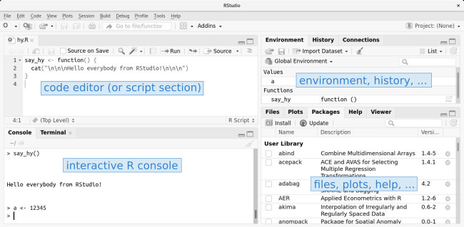
The interface consists of a code editor (“text” editor; top left), the R command line (bottom left), a summary of your current workspace (might be empty; shows all objects defined in the current R session; top right) and access to plots, help pages, and packages (bottom right).
- Code editor: The code editor, or script section, is used to write scripts (programs).
- R console: This is where the magic happens. The R console is interactive, we can directly enter and execute commands here, or we write our script in the code editor and “Run” the script which will then be executed “line-by-line” in the R console (shown later). You will see the output of your script down here (results, warnings, error messages, …).
- Envornment/history: Shows all objects defined on your current “workspace”. If you just installed R right now, this part should be empty. Furthermore, the “history” tab allows you to see the last commands you executed.
- Files, plots, help: This area is used to show files, plots (if we plot something), or show links to help and manual pages. We will come back to this, soon.
3.1 Entering commands
Let us start with executing our first commands in the interactive R console (bottom left). This is the area you “communicate” with R. do. Whenever you enter something and press the “Enter” key it will be executed by R. Everything we enter here is called “a command”. A command is a simple instruction which tells R what to do. For example:
- calculate the result of five times 2:
5 * 2, - call a function to create an integer sequence:
seq(10, 100, by = 10), - or more complex calls such as plotting some random numbers:
plot(rnorm(400), main = "Random Numbers")
The R console is mainly used for interactive tasks, e.g., interactively analyzing some data or to test a command and see if it works. As soon as starting with “more complex” tasks we will write scripts (will be explained in a minute).
R as a basic calculator
Let us start simple and use R as a basic calculator.
We would like to find out what
5 to the power of 2 is (\(5^2\)). It is obviously 25, but let R do the
calculation for us. All we have to do is to enter the following in the R console:
In R the ^ operator is the power operator, 5^2 thus calculates 5 to the power of 2.
Well, that’s your first command! As soon as you let it run (press “Enter”) R does the
math and returns the result which will be shown in the R console window.
## [1] 25As expected, \(5^2 = 25\). But what does the rest of the output tell us? ## is used in this
documentation/book to indicate that this is “the output generated by R”, you will not see
this in your RStudio session. However, you’ll see the [1]. [1] tells us that
the first number returned by R was 25 and is only an indicator and not part of the actual
result.
R as an advanced calculator
We can, of course, do more than that. Let us start using R as an advanced calculator using some variables or objects.
We will do the same and calculate \(5^2\), but this time using a variable.
Rather than simply writing 5^2 we will calculate a^2. To be able to do so,
we first have to create a variable (or object) a and assign the value 5 to it.
This can be done as follows:
The two lines above tell R to store the value 5 on a variable a. If a
already exists, it simply overwrites it. Thus, the two lines above will not
create two different a’s as the second line overwrites our first a.
The only difference between the two lines is that we once use = and once
<-. The latter one is called the “gets operator” in R and is the
preferred way to assign data to variables or objects. The = works the same
way most of the time, but we’ll try to stick to the gets operator from now
on!
Note: if you now check your Workspace (Environment, top right panel in RStudio)
there should now be an entry “a”. This tells us that we have defined a variable a
which we can now use in our calculation. If you simply enter a in
the R terminal you should see this:
## [1] 5By default, R prints the content of an object (variable) if we just enter the
name of the object (here a). This is called implicit printing. We can, of course,
also use explicit printing by calling print(a):
## [1] 5… which gives us the very same result. An alternative way to (i) assign some
values to an object (again a) and implicit printing at the same time is to
put another pair of round brackets around it. Not the best way, but you may see
it every now and then:
## [1] 4321Note: implicit printing is only
used when you are working on an interactive R console (as in your IDE). When
you want to print within a script (see below) you have to do explicit printing:
More than that, we can now also use our object a to do some calculations.
Let’s see what a^2 is:
## [1] 18671041Let’s assume that we don’t want to solely compute \(5^2\) but do the same operation for a sequence of numbers (\(1^2\), \(2^2\), \(3^2\), …). A sequence of numbers is called a vector (we will learn “everything” about vectors in the chapter Vectors).
E.g., c(1, 2, 3) is a vector
which contains three different numeric values, 1, 2, and 3.
Let’s first specify a new variable we call b which should contain a
set of numbers between 0 and 30. We can use the function seq(...)
which returns us a sequence of values between two limits (from … to).
##  [1]  0  1  2  3  4  5  6  7  8  9 10 11 12 13 14 15 16 17 18 19 20 21 22 23 24
## [26] 25 26 27 28 29 30
The first line creates the sequence and assigns (<-) it to a new variable b,
the second line prints b. Remember the [1] from above? In this case we do have
two indicators, namely [1] and [26]. Again, this is not part of b
but helps you to interpret the output.
[1]: the first line starts with the first element of our vector/sequenceb.[26]: the second line starts with the 26th element of our vector/sequenceb.
We could now take each element to the power of two (let’s say calculate \(0^2\),
\(1^2\), …) element by element which, at least by hand, will take quite some
time. In R (as in other programming languages) we can also perform this
calculation on a vector which solves it element-wise.
Thus, b^2 will take each element of b to the power of 2.
##  [1]   0   1   4   9  16  25  36  49  64  81 100 121 144 169 196 225 256 289 324
## [20] 361 400 441 484 529 576 625 676 729 784 841 900
The result is of the same length as b but each element is now taken to the
power of 2. As we do not assign the result to a variable, R only prints the
result (b^2). To store the result we have to assign it to a new variable. Let’s
call the new variable result and store b^2 onto it:
##  [1]   0   1   4   9  16  25  36  49  64  81 100 121 144 169 196 225 256 289 324
## [20] 361 400 441 484 529 576 625 676 729 784 841 900
This is what we will typically do (store the result of a command we execute) such that we can use it for further calculations, plotting, or to save the results into a file. If you only print it (no matter whether it is implicit or explicit printing) the values will get lost.
First basic plot
R also provides a wide range of nice functions to plot data. We will learn
more about how to plot data in another chapter, but to demonstrate how a very
basic plot could look like we quickly visualize b^2 as follows:
plot(b, b^2)
lines(b, b^2, lty = 2)
lines(b, b, col = 2)
legend("topleft", legend = c("b^2", "b"), col = c(1, 2), lty = c(2, 1), pch = c(1, NA))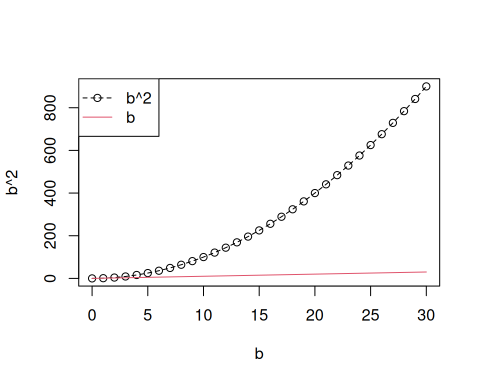
3.2 The + on the console
One important little thing to mention: If you see + at the start of a line on
the R console like this …
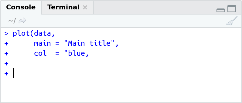
… it means that you have entered (run from script or directly entered) an
incomplete command! The + indicates a “follow-up” line and R is actually
waiting for you to finish and close the command.
In the example above I wanted to plot something and call the plot function. Function calls
always need an opening bracket (() and a closing bracket ()) (will be discussed in
chapter Functions). In the example we open the
bracket ((), specify some inputs to the function but never close the call () missing).
You can either finish the command or press ESC (Escape) to interrupt.
3.3 Working directory
You are, for sure, all familiar to the structure of files and folders on your computer as you all have some kind of a “Documents”, “Desktop”, and “Downloads” folder, maybe a folder for “Photos” and/or a folder to store your personal “Music” library.
On all computers, files are stored/ordered in a similar way except that the file paths look a bit different. Example paths:
- Windows: “
C:/Users/Miriam/Downloads” - OS X: “
/Users/miriam/Downloads” - Linux: “
/home/miriam/Downloads”
When working with files in R, e.g., load data from the disc, source script files, store images, … we do have to consider “where we are right now”. “Where we are right now” is a very sloppy expression of what is called the current working directory.
For different tasks we will use R data sets stored in files. As an example, let us import a data set which contains some information about all municipals (Gemeinden) in Tirol. First, we need to download the data set and store it on our computer.
- Click on the file name to download "tirol.rds".
This data set comes in the ‘RDS’ file format, we will learn more about it
in the chapter about Reading & Writing).
For now, all we need to know is that we can import this data set using
the function readRDS(). To read the file, we call:
## Warning in gzfile(file, "rb"): cannot open compressed file 'tirol.rds',
## probable reason 'No such file or directory'
## Error in gzfile(file, "rb"): cannot open the connectionAll we get is an error message! Why? Well, R simply cannot find the file
"tirol.rds" (No such file or directory).
Either the file does not exist at all, or R the file is stored somewhere
where R cannot find it right now. Our file argument is ‘just’ a file name
(thus a relative path) and R expects the file to be located in the current
working directory.
Current working directory
In R studio your current working directory is always shown in the top part of the R console:
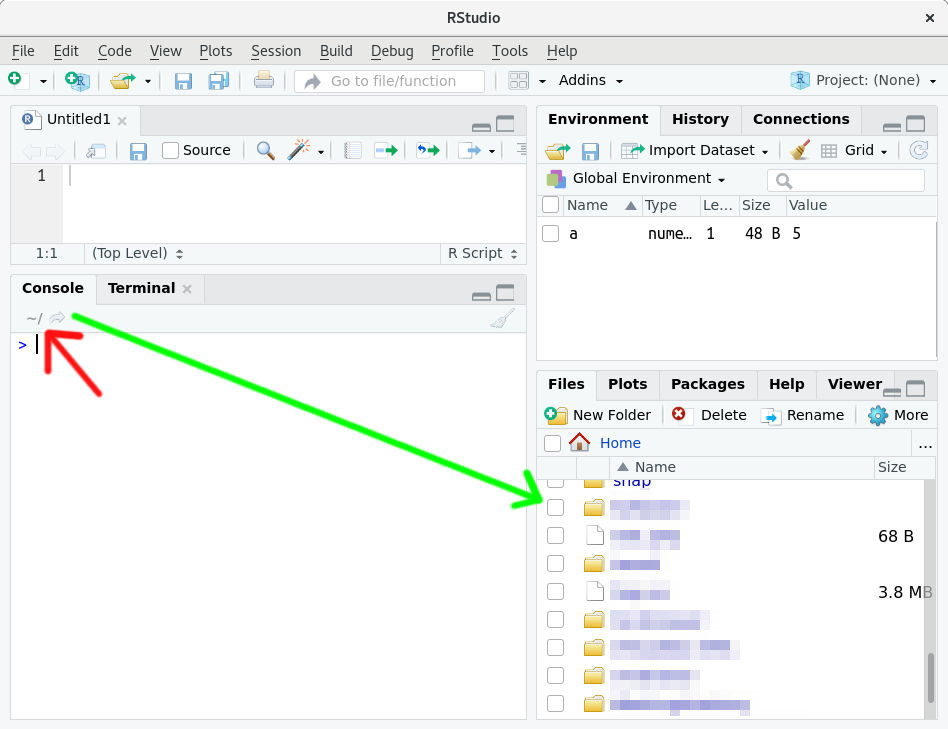
Figure 3.1: Where to find your current working directory (red arrow).
In my case it is simply “~” (red arrow) which is the
user home directory on Linux. If you click the small arrow-icon just next to
it, the content of the current working directory will be shown in the bottom
right corner (green arrow).
Alternatively, we can use the function getwd() to ‘get working directory’.
This also shows the current working directory. As our data set ("tirol.rds") is
not located here, R cannot find it. To get the data set loaded, we need to
change it.
Change working directory
We could, of course, solve the problem by simply copying the file
"tirol.rds" file into the current working directory (here the home
directory), however, that’s not a good option as you would end up with storing
everything in your home directory.
Another solution would be to use absolute paths to read the file. In contrast to relative paths (relative to the current working directory) absolute paths specify the full path relative to your system.
Let’s say your user on your computer is “Miriam”, then we could do something like:
readRDS("C:/Users/Miriam/Downloads/tirol.rds")on WindowsreadRDS("/Users/Miriam/Downloads/R-course/tirol.rds")on OS XreadRDS("/home/Miriam/Downloads/R-course/tirol.rds")on Linux
… but that’s not a good option either! Why? Imagine you write a program
which uses absolute paths (e.g., solution for homework) - and then send this
script to me. I will not be able to run your code as the directory
"C:/Users/Miriam/Downloads" simply does not exist on my computer.
Not even "C:/" as this is Windows-specific. Thus, always try to avoid absolute
paths!
An additional advice (not only for programming in R, but in general) as it will, sooner or later, cause problems:
- Do not use special characters in folder/file names (bad:
"Bevölkerungszahlen_Österreich.R") - Do not use blanks either (very bad:
"Bevölkerungszahlen Österreich 2018-2019.csv")
But back to R. What we will do instead is to properly set the working directory.
In RStudio you can do this in several ways. The simplest way: go to
“Session > Set Working Directory > Choose Directory” (or shortcut CMD+Shift+H/Ctrl+Shift+H):
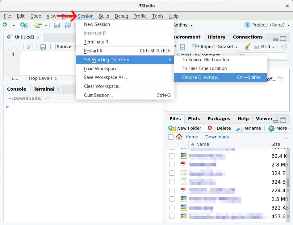
Figure 3.2: Change working directory for the current RStudio session.
A new window will open where you can navigate to the folder which should be your
new working directory (e.g., "C:/Users/Miriam/Downloads", "/home/miriam/Downloads")
where your file is located and and press “Open”.
Alternatively we can also set the current working directory using the R function setwd()
(set working directory). Simply call something like:
… which does the very same as the procedure described above. After changing
the directory you will see that the path in the header of the R console tab
changes (in the screenshot to ~/Downloads). As we are now in the correct
folder where our data set is located, we can again call:
##            Name Hoehe Flaeche Einwohner
## 1 Abfaltersbach   983   10.30       643
## 2         Absam   632   51.92      6993
## 3    Achenkirch   916  114.01      2215
## 4         Ainet   747   40.46       923
## 5       Aldrans   760    8.86      2661
## 6       Alpbach   974   58.41      2559
And can finally read the data set. head(tirol) shows the first few entries
of the data set, something we will learn more about in the next chapter.
Keep in mind: Whenever R throws an error message like “cannot open the connection”: check your working directory, that you have not misspelled the file name, and if the file really exists.
3.4 Our first script
So far, we have just entered one command after another. As soon as things are getting more complex, entering line-by-line every time is neither efficient nor what you want to do. Instead, we will write a so called script.
A script is the natural extension of commands and nothing else than a sequence
of commands stored in an .R file. We could also call a script a (simple)
computer program, however, “a program” is not very specific and could basically
be everything. R, as most other programming languages, execute scripts
sequentially line-by-line. A small well-written script could look as follows:
# ---------------------------------------------
# Name:        create_thesis_graph.R
# Author:      Reto Stauffer
# Date:        2017-04-04
# Description: Small script to create the
#              figures for my bachelors thesis.
# ---------------------------------------------

# Clear workspace (deletes all existing user objects
# and user functions).
rm(list = objects())

# Import data set
tirol <- readRDS(file = "tirol.rds")

# Extract municipals with more than 10000 inhabitants (Einwohner).
tirol <- subset(tirol, Einwohner > 10000)

# Create a barplot with all municipals larger than 10000 inhabitants.
# 1) We store the graph as a PDF image; pdf(...) opens the PDF.
# 2) Create a barplot
# 3) Close/write the PDF by calling dev.off()
pdf(file = "thesis_figure_001.pdf", width = 10, height = 5)
    barplot(height = tirol$Einwohner,
            names.arg = tirol$Name,
            main = "Municipals with more than 10k Inhabitants")
dev.off()
Note: we don’t have to understand all the details, that’s what we will learn step-by-step together in this book.
Content of a script
- Meta information: The script should contain meta information (the comments in the first few lines) which tells us how where we stored the script, who wrote it, and a small description what the script does. Note: that this is not mandatory, but we recommend to include some meta information as you will quickly forget why you wrote the script.
- Instructions and comments: The rest of the script contains commands and comments. The comments are only for us humans (again, R does not need them) which help you to (i) structure your script and (ii) remember why you did what and why. In this case: read a file, subset the data, and create a plot. We will learn about the commands here in some of the other chapters.
Important: Scripts should always be executable! That means that one should be able to run the script from A-Z without running into errors. Thus, take care that, if you write a script, that there are:
- no incomplete statements (Refresher)
- things where you tried out some code which does not work at all
- commands which result in an error (R will stop execution on errors)
- calls to open R documentation (help pages) such as
?meanorhelp("load") - simple “text” which should actually be comments
- …
Create first script
To do so, we will use the code editor in RStudio which is the top left
window (if not minimized). What we have to do first is to open a new
R script.
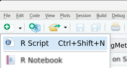
A new script can be created by clicking “R Script” under icon with the small
green plus in the top left corner of RStudio (or use CTRL+SHIFT+N, or via
“File > New File > R Script”).
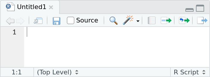
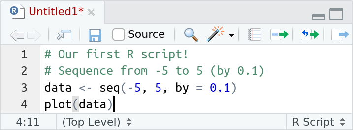
Once you did that you will see a new empty window which currently has no name or title (tab says “Untitled*”).
In this window, we can now start to write our script. A simple example is the following which creates a numeric sequence and plots it.
Comments
Lines starting with a # and everything behind a #
are comments. Comments are ignored by R (not executed). Even if comments do
not affect what is executed, comments are an essential part of scripts/programs
and are used to describe what is going on, or why you did something.
## [1] 25## [1] 0.1239031Comments can also span multiple lines (each line has to start with #) for
more information/larger descriptions or to separate different parts of a
script. We will see that when writing longer scripts.
Keep in mind that code is more often read than written! Well written comments will make it much easier for you to understand what you did and why you did it (believe me, you will forget it) but also for others checking, using or adapting your code. Some people say a good code-to-comment ratio is 60 percent comments, 40 percent code.
Save script
WARNING: An important warning first for Windows users. Windows 10 does not allow us to store R scripts into the “Documents” folder! We suggest you to create a new directory (outside ‘Documents’) and call it “R-course” or something similar.
RStudio informs us that we have not yet saved our script (highlights the name of the tab in red). Thus, remember to store your script soon enough (best: immediately) not to loose your progress.
To save the script, simply press the “Save icon” (or “File > Save”).
R scripts are stored in “.R” files, e.g., “homework_03.R”. I would recommend
that you create yourself a folder somewhere for this course where you can store
the script files and data sets we will use in the next chapters.
Hint: use meaningful file names (will be discussed in another chapter).
Bad naming:
foo.R,foo2.R,foo3.Rtest.R,test_2.R
Good names:
homework_03_malaria.Rthesis_analize_sales.Rthesis_generate_results_plots.R
Once saved, you can see the script file name (title). Note: R script files are basically just ASCII text files with commands, you can also easily send them to someone else, backup them, …
Run scripts
Last but not least, we need to execute the script. We have several options (RStudio):
- Execute specific lines/sections from the script,
- execute the script “line-by-line”,
- or execute the whole script in one go.
To execute one specific line: we simply click into the line we would like
to execute and press the button with the green arrow (“execute current line or selection; or CTRL+ENTER).
RStudio will copy this line into the R console and execute the line (as if we would enter
the command and press enter). The mouse cursor in the code editor is then placed in the next line.
Execute a selection: As for single lines: use the mouse to select multiple lines and press
the icon with the green arrow (or press CTRL+ENTER).
Execute script line by line: Often nice when developing code. This is the very same as execute one specific line.
- Select the first line you would like to execute (place the mouse cursor there)
- On your keyboard: press
CTRL+ENTER. The line will be executed, the cursor jumps into the next line. - Again, press
CTRL+ENTERto execute the next line … and so far, and so on.
Execute the whole script: We can also run the whole script with one click.
The icon with the blue arrow says “execute the content of the active script”.
If you press it, you’ll see that, in the R console the command source("<file name>.R")
shows up.
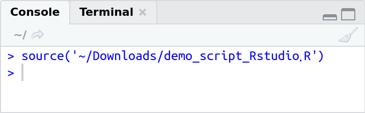
source("<file name>.R") is the command which executes the whole script file.
If your script generates output (uses explicit printing; print()) or runs
into errors or warnings, you will see the output here.
Multi-line, blank lines
Commands can also be spread over multiple lines. The example below shows that
the plot(...) command is split up over 3 lines.
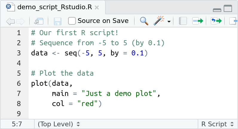
This is often useful (and recommended) if you have long commands. The screen-shot above also shows that the script contains blank lines: blanks are often used before a comment/after a command to separate different “blocks” or “chunks” from each other an to increase the readability.