Chapter 11 Data Classes & Methods

Construction of complex objects

So far we have a series of different data structures/objects including vectors, matrices, lists and data frames. We have learned that ‘more complex objects’ (matrices; data frames) are all based on the most basic objects (vectors; lists). This idea can be used to create a variety of additional (even custom) data classes for specific purposes.

Generic functions

We observed that the behaviour of a function may depend on a class of an object we call it for. This happens for generic functions, such as:

print(), str(): presenting an object in a way which is meaningful for its content.
summary(): showing a summary of characteristics specific to an object.
plot(): creating a plot suitable for particular objects (single vector, two vectors, formula, data frames).

Besides these four examples, a range of additional generic functions exist. If we need something very specific for our own work we can also create custom classes and methods for specific data types or define additional generic functions (if needed). This is relatively easy once we understand how it works in R.

Goal of this chapter

In this chapter, we will learn about two additional data structures in R. One for categorical data (factor) and date-time objects (Date, POSIXt). First, factors are introduced and ‘deconstructed’ to see how an object of class factor is constructed. This helps to understand how generic functions work and allows us to write our first own custom class. To back this up we will learn how date and date-time objects in R work and how they are constructed.

11.1 Categorical data (factors)

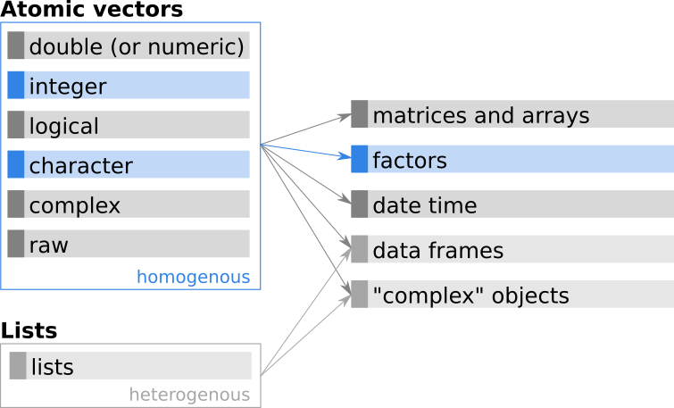
Figure 11.1: Additional base R classes based on atomic vectors.

Categorical data are used for qualitative variables when the outcome of a specific observation/measurement falls into (exactly) one of a number of known and countable categories.

Clarify the jargon: In R, objects for categorical data are called factors, while the different categories in which an observation can fall is called a level. Other programming languages/software may use different labels, e.g., ‘Enumerated Type’ (ENUM) in SQL/MySQL databases, C/C++, and JAVA, or ‘category’ in Python pandas.

Binary examples: Only two distinct outcomes (two possible categories).

	Description	Levels
Nominal	Precipitation	`"rain"`, `"no rain"`
	Power supply	`"on"`, `"off"`
	Purchase of a product	`"yes"`, `"no"`

Examples with $\ge 3$ categories: When having more than two possible outcomes, one talks about categorical data (whereof binary is a special case). Categorical data can be nominal (unordered) or ordinal (ordered). Ordered means that we can bring the categories in a distinct order, which can not be done for nominal data.

	Description	Levels
Nominal	Gender	`"female"`, `"male"`, `"diverse"`
	Blood type	`"A"`, `"B"`, `"AB"`, `"0"`, …
	Means of transport	`"bike"`, `"car"`, `"train"`, …
Ordinal	Education	`"bachelor"`, `"master"`, `"phd"`
	Satisfaction	`"low"`, `"medium"`, `"high"`
	Rating	`"AAA"`, `"AA+"`, `"AA"`, …

Nominal versus ordinal:

Gender (nominal): We cannot bring ‘gender’ into a specific order, males are not ‘below/above’ females or diverse persons.
Education (ordinal): The three categories ‘bachelor’, ‘master’, and ‘phd’ can be brought in a distinct order. We cannot get a Masters degree as long as we have not finished our Bachelors study. And we need a Masters degree first to finish our PhD (doctorate).

Creating factors

Factors can be created using the function factor() (the constructor function). From the documentation:

factor(x = character(), levels, labels = levels,
       exclude = NA, ordered = is.ordered(x), nmax = NA)

Important arguments:

x: a vector of data, usually taking a small number of distinct values.
levels: an optional vector of the unique values (as character strings) that ‘x’ might have taken. The default is the unique set of values taken by ‘as.character(x)’, sorted into increasing order of ‘x’.
labels: either an optional character vector of labels for the levels (in the same order as ‘levels’ after removing those in ‘exclude’), or a character string of length 1. Duplicated values in labels can be used to map different values of x to the same factor level.
exclude: a vector of values to be excluded when forming the set of levels. This may be a factor with the same level set as x or should be a character.
ordered: logical flag to determine if the levels should be regarded as ordered (in the order given).

From character vector

When a factor is created from a character vector, all unique values of the vector are taken as levels (categories), the categories are lexicographically sorted.

Let us create a character string which contains the educational attainment of a series of people, coded by the highest university degree.

(degree <- c("master", "master", "bachelor", "phd", "bachelor", "master"))

## [1] "master"   "master"   "bachelor" "phd"      "bachelor" "master"

class(degree)

## [1] "character"

This is a classical categorical variable: We have 6 observations (or elements), but only 3 possible levels (categories). Thus, let us convert this character string into an object of class factor.

(degree <- factor(degree))

## [1] master   master   bachelor phd      bachelor master  
## Levels: bachelor master phd

class(degree)

## [1] "factor"

The object degree is now of class factor and the representation of the object changed – not only the quotation marks are gone (""s), we also get an additional line with Levels. Each outcome of our original character vector is taken as one of the levels, lexicographically sorted (try sort(unique(degree)) on the character vector).

Plotting factors & numerical summary:

Before going into more detail let us see why factors are useful. Let us have a look at the numerical summary (summary()).

summary(degree)

## bachelor   master      phd 
##        2        3        1

As R recognised that we have categorical variables we now get absolute counts (as from table()). The same if we use the generic function plot(). As a line plot would not be meaningful, R automatically draws a bar plot.

plot(degree, col = "steelblue")

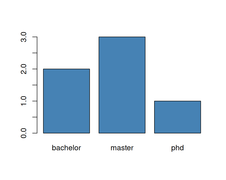
As you can see, factors help us a lot when dealing with categorical data.

Basic properties and attributes:

Properties: Like all objects, factor objects always have a length, and a type.
Attributes: Factor variables always have two attributes, a class (factor) and an attribute levels.

Let us investigate the object degree from above.

list(class  = class(degree),
     typeof = typeof(degree),  # <- !!!!
     attributes = attributes(degree))

## $class
## [1] "factor"
## 
## $typeof
## [1] "integer"
## 
## $attributes
## $attributes$levels
## [1] "bachelor" "master"   "phd"     
## 
## $attributes$class
## [1] "factor"

While the class is as expected, typeof() returns us integer. Keep this in mind (will become clear later). In addition, we can see that we have the two (mandatory) attributes "class" (simply "factor") and "levels", the character labels (names) of the different levels/categories.

Dedicated extractor functions: For factor variables, a series of extractor functions exist we have not seen so far.

levels(): Extracts the character labels (levels); returns a character vector.
nlevels(): Returns the number of different levels; single integer.

list(levels = levels(degree),
     nlevels = nlevels(degree))

## $levels
## [1] "bachelor" "master"   "phd"     
## 
## $nlevels
## [1] 3

Extracting attributes: In the meantime we learned how to work with lists. And we know that all attributes of R objects are stored as a named list (check the output of attributes()).

We can access attributes by using attr(x, which) where x is the target object, and which the name of the attribute, or by using attributes(x) (returns named list). Thus, we could also use the following commands to get the same information as levels() and nlevels() using:

# Extracting levels (two different ways)
attr(degree, "levels")

## [1] "bachelor" "master"   "phd"

attributes(degree)$levels

## [1] "bachelor" "master"   "phd"

# Number of levels
length(attr(degree, "levels"))

## [1] 3

length(attributes(degree)$levels)

## [1] 3

Note: It’s recommended to use the dedicated extractor functions (here levels() and nlevels()) if available.

Structure of a factor: Let us have a closer look to the structure of a factor object and how it is constructed.

str(degree)

##  Factor w/ 3 levels "bachelor","master",..: 2 2 1 3 1 2

As shown, we get the information that we have a factor variable with (w/) 3 levels; followed by names of the first few levels. What about the integer values at the end of the output?

Let us use a new function called unclass(). It removes the class of an object and deconstructs it to the simplest possible object, a vector (atomic vector) or list (generic vector).

unclass(degree)

## [1] 2 2 1 3 1 2
## attr(,"levels")
## [1] "bachelor" "master"   "phd"

We can now see how the object is constructed. A factor object is nothing else than an integer vector ([1] 2 2 1 3 1 2) with an additional attribute levels containing the names of the three levels. This is nothing else as a ‘lookup table’. The integer vector (index vector) tells us that the first entry of our object belongs to category 2, the second to category 2 and so far and so on.

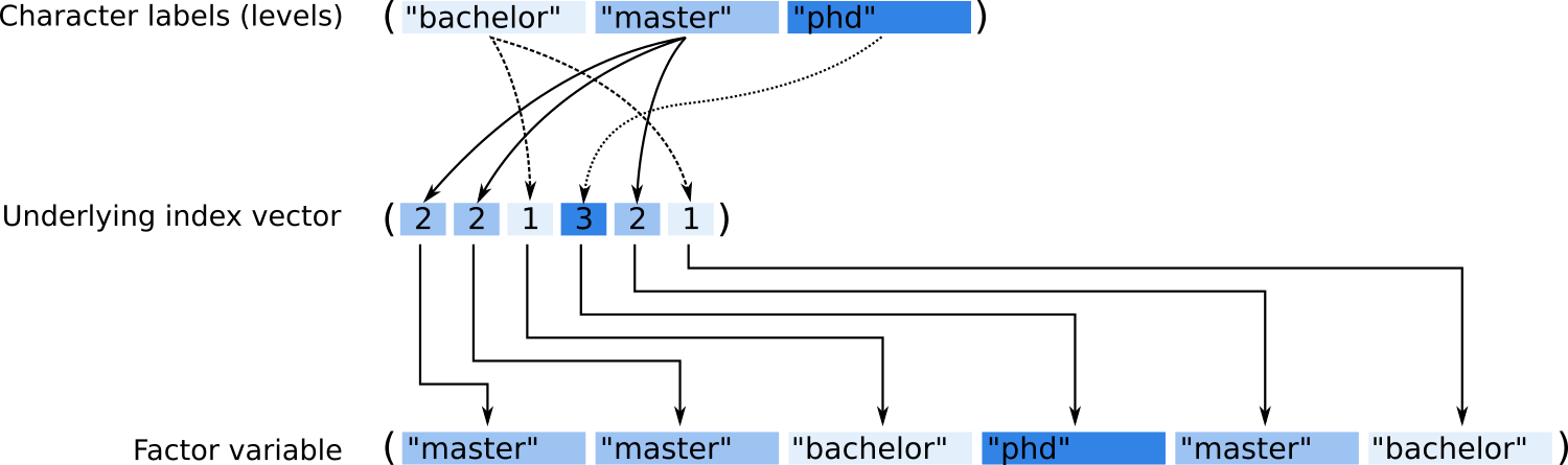
Figure 11.2: Graphical representation of the internal structure of a factor variable.

As our factor variable is indexed by index values (our integer vector), we can also use this for subsetting. An example:

c("BSc", "MSc", "PhD")[degree]

## [1] "MSc" "MSc" "BSc" "PhD" "BSc" "MSc"

… this is nothing else than subsetting by index (see Vectors: Subsetting by index).

By hand: Let us do c("BSc", "MSc", "PhD")[degree] ‘by hand’ to better understand what’s going on.

Crate yourself a new object new_names <- c("BSc", "MSc", "PhD") (character vector)
Coerce (convert) degree to integer using explicit coercion, store result on idx.
Use idx and new_names to create the same as shown above.

Solution. Let us create the new character vector and the idx object in the first code chunk. The coercion is done using as.integer(degree).

new_names <- c("BSc", "MSc", "PhD")
(idx <- as.integer(degree))

## [1] 2 2 1 3 1 2

We can now use idx to subset by index as follows:

new_names[idx]

## [1] "MSc" "MSc" "BSc" "PhD" "BSc" "MSc"

… and that’s exactly what is shown above:

c("BSc", "MSc", "PhD")[degree]

## [1] "MSc" "MSc" "BSc" "PhD" "BSc" "MSc"

Summary:

The number of categories (levels) is fixed.
Character labels (names) of the levels/categories are stored as attribute "levels".
The data are indexed by an integer vector (a factor object is an integer vector with an attribute levels).
The separate class (factor) allows the creation of dedicated methods for categorical data such as subsetting, visualization, modelling, …

From integer vector

Instead of starting from a character vector, we can also create factor variables based on an integer vector. This is often useful when we have a data set at hand which contains categorical information coded as integers as in the following example.

# Integer coding:
# 1 = bachelor
# 2 = master
# 3 = phd
(degree2 <- c(1L, 3L, 1L))

## [1] 1 3 1

# Convert to factor variable
(degree2 <- factor(degree2,
                   levels = 1:3,
                   labels = c("bachelor", "master", "phd")))

## [1] bachelor phd      bachelor
## Levels: bachelor master phd

As shown in the comments, we know that this data set may contain three possible categories. Level 1 corresponds to "bachelor", 2 to "master", and 3 to "phd". The two arguments levels and labels define this connection and are used to convert our integer vector into a proper factor variable.

Note: We have defined three possible outcomes, even if the data set itself only contains two of them (we have no 2 = master).

Creating ordered factors

So far we always had nominal data (unordered). If the order of the different categories is important, we can set the additional argument ordered to TRUE. The rest is the very same as above, however, the output does look different:

# Calling the object 'odegree' (ordered degree)
(odegree <- factor(c(1L, 3L, 1L),
                   levels = 1:3,
                   labels = c("bachelor", "master", "phd"),
                   ordered = TRUE))

## [1] bachelor phd      bachelor
## Levels: bachelor < master < phd

As shown, we now get Levels: bachelor < master < phd; The ‘smaller then’ operator (<) indicates that the categories are now ordered (from left to right). This adds some additional functionality:

odegree[1] < odegree[2]

## [1] TRUE

odegree[1] > odegree[2]

## [1] FALSE

… which will not work on nominal (unordered) factors. In addition, such ordered factors can be very useful when estimating statistical models (not part of this course).

Factors from continuous numeric

Another very handy function is cut(). It allows us to create a categorical variable (factor) based on defined intervals based on a continuous scale (numeric vector).

Usage:

cut(x, breaks, labels = NULL,
    include.lowest = FALSE, right = TRUE, dig.lab = 3,
    ordered_result = FALSE, ...)

Important arguments:

x: a numeric vector which is to be converted to a factor by cutting.
breaks: either a numeric vector of two or more unique cut points or a single number (greater than or equal to 2) giving the number of intervals into which x is to be cut.
labels: labels for the levels of the resulting category. If FALSE integer codes are returned (instead of factor).
ordered_result: logical: should the result be an ordered factor?

Example: We would like to classify the state of water given a specific temperature in degrees Celsius. Below $0$ degrees Celsius "solid", $0 > x \le 100$ degrees Celsius as "liquid", and $> 100$ degrees Celsius "gas".

We can specify the breaks (where to cut the continuous variable) using the breaks argument. If set to a single integer, R selects some breaks (e.g., 8 breaks). In case we know where to cut, as in this example, we can define a numeric vector (on breaks) defining these break points.

temp <- c(17.5, -4.3, 36.0, 68.1, 130.0)  # observations
cut(temp,
    breaks = c(-Inf, 0, 100, Inf),        # 4 breakpoints = 3 segments
    labels = c("solid", "liquid", "gas")) # 3 labels (categories)

## [1] liquid solid  liquid liquid gas   
## Levels: solid liquid gas

Take care: if we have 4 breaks we define 3 segments (categories) and therefore only need 3 labels. If no labels are specified, R will set default levels of the form (a, b] (mathematical definition of an interval). The excursion below (not mandatory) shows more details on that for those interested.

By default, the levels are set to (a, b] which mathematically defines a ‘left open, right closed’ interval. This simply means that this interval includes all numbers $a < x \le b$ ($a$ not included; $b$ included). In our example, an observation falling on 0 would fall into the first segment, those on 100 into the second segment.

This can be changed by setting right = TRUE creating ‘left closed, right open’ intervals.

cut(temp, breaks = c(-Inf, 0, 100, Inf), right = TRUE)

## [1] (0,100]    (-Inf,0]   (0,100]    (0,100]    (100, Inf]
## Levels: (-Inf,0] (0,100] (100, Inf]

In addition: the lowest (or largest if right = TRUE) value will be ignored except you set include.lowest = TRUE. This can be crucial as well but is no problem in this example, as the outer bounds have been set to -Inf, and +Inf.

# Using absolute 0 (0 Kelvin) as the lower bound,
# Include lowest (in case it would be -273.15).
(state <- cut(temp,                                  # numeric values
              breaks = c(-273.15, 0, 100, Inf),      # 4 breakpoints
              labels = c("solid", "liquid", "gas"),  # 3 labels (categories)
              include.lowest = TRUE,                 # include lowest (-273.15 as 'solid')
              ordered = TRUE))                       # ordered categories

## [1] liquid solid  liquid liquid gas   
## Levels: solid < liquid < gas

list(class      = state,
     levels     = levels(state),
     nlevels    = nlevels(state),
     is.ordered = is.ordered(state))

## $class
## [1] liquid solid  liquid liquid gas   
## Levels: solid < liquid < gas
## 
## $levels
## [1] "solid"  "liquid" "gas"   
## 
## $nlevels
## [1] 3
## 
## $is.ordered
## [1] TRUE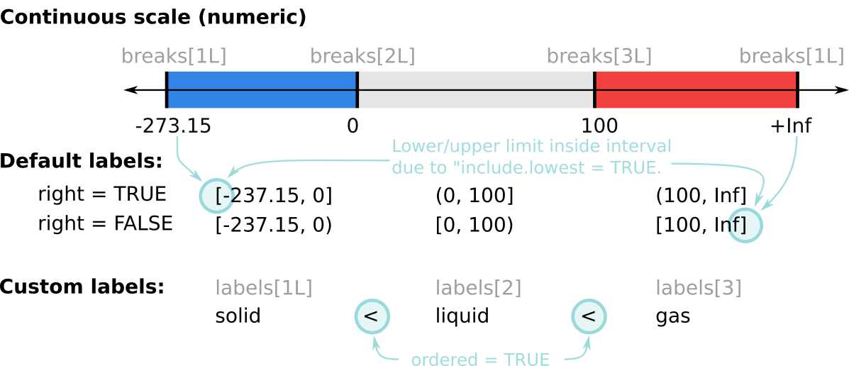

Figure 11.3: Graphical representation of the function cut(); three intervals (-273.15 to 0, 0 to 100, and 100 to +Inf).

Subsetting and replacing elements

Factor variables allow for proper subsetting or to replace specific elements, the same as for vectors. This includes subsetting by index, subsetting by logical vectors, and even subsetting by name (it is technically possible to add names to the elements of a factor; not seen often).

Subsetting by index: Extract the first element, and elements c(6, 3) (in this order). The result is still a factor, all levels are kept.

degree[1]

## [1] master
## Levels: bachelor master phd

degree[c(6, 3)]

## [1] master   bachelor
## Levels: bachelor master phd

Subsetting by logical vectors: Straightforward.

degree[c(TRUE, TRUE, FALSE, FALSE, FALSE, FALSE)]

## [1] master master
## Levels: bachelor master phd

Replace elements: We can also assign levels and overwrite specific elements. Note: Only works for defined levels!

degree[5] <- "bachelor"       # replaces element 5
degree[6] <- "habilitation"   # won't work, not a valid level!

## Warning in `[<-.factor`(`*tmp*`, 6, value = "habilitation"): invalid factor
## level, NA generated

Subsetting and replacing levels

In the same way, we can also subset or replace (specific) levels and change the names of the categories if needed.

levels(degree)[1]

## [1] "bachelor"

levels(degree) <- c("BSc", "MSc", "PhD")
degree

## [1] MSc  MSc  BSc  PhD  BSc  <NA>
## Levels: BSc MSc PhD

Reference category, unused levels

Sometimes it is necessary to have a very specific category as the first level in your factor object, e.g., when estimating statistical models. This first level is called the reference category or reference class. Furthermore, it might sometimes be useful to remove (drop) unused levels. The following excursion (not mandatory) shows how this can be done for those who want to know.

We know that, by default, the levels of a factor are lexicographically sorted (if not ordered). Imagine you perform a medical experiment testing some drugs. The participants either get the “standard” treatment, the “new” treatment, or a “placebo” medication (with no effect).

(drug <- factor(c("placebo", "new", "placebo", "standard", "new")))

## [1] placebo  new      placebo  standard new     
## Levels: new placebo standard

Our first level is new, but we want placebo as the first level as this is our reference category (ref; first category/level). This is often important when using such data for statistical modelling (beyond this course). To define placebo as our first category, we can use relevel().

(drug <- relevel(x = drug, ref = "placebo"))

## [1] placebo  new      placebo  standard new     
## Levels: placebo new standard

Drop unused levels

In case you have unused levels and you want to drop them, call droplevels(). Let us take the example from above with c("bachelor", "master", "phd") where we have not had any master student (see From integer vector):

(degree2 <- factor(c(1L, 3L, 1L),
                   levels = 1:3,
                   labels = c("bachelor", "master", "phd")))

## [1] bachelor phd      bachelor
## Levels: bachelor master phd

Let us drop all unused levels: the result is a factor object with only two levels ("bachelor", and "phd").

droplevels(degree2)

## [1] bachelor phd      bachelor
## Levels: bachelor phd

Note: For unordered factors (orderered = FALSE;, default) droplevels(degree2) does the very same as factor(degree2). droplevels(degree2) is a convenience function which, internally, calls factor().

What factor(degree2) does: it converts the input (degree2) into a character vector (explicit coercion), and creates a new factor object out of it.

If we have a level but no observation assigned to this level/category, it will not be included in the character vector. Thus, when creating a new factor out of it, it will be dropped. By hand:

# 'by hand'
(test <- as.character(degree2))

## [1] "bachelor" "phd"      "bachelor"

factor(test)

## [1] bachelor phd      bachelor
## Levels: bachelor phd

# Which is the same as
factor(degree2)

## [1] bachelor phd      bachelor
## Levels: bachelor phd

# Which does the same as
droplevels(degree2)

## [1] bachelor phd      bachelor
## Levels: bachelor phd

For ordered factors this will not work as as.character() converts our data into a bare character vector – wherefore we will again end up with lexicographically ordered levels.

Methods for factors

Question: We have now seen what we can do with factors. But is this really necessary? I mean, couldn’t we simply take an integer or character vector and have the very same information?

Answer: Yes, but there are many advantages of having a dedicated class for categorical data and R provides a series of methods for data handling (e.g., coercion, subsetting, visualization, …).

Let us highlight the differences between a pure integer vector, a character vector, and a factor object (containing the ‘same’ information). To do so, we first coerce our factor degree into a pure integer vector (degree_int) and a character vector (degree_chr).

degree <- factor(c("master", "master", "bachelor", "phd", "master", "bachelor"))
degree_int <- as.integer(degree)     # coerce to integer
degree_chr <- as.character(degree)   # coerce to character

We will then use the generic functions print(), summary() and plot() to highlight the advantages: The good, the bad, and the ugly.

The good

print(): Easy to read as all values are coded with their corresponding category. In addition, we see what categories we have.
summary(): As we have counts, the numerical summary shows us how many observations we have in each class (absolute counts; as table()).
plot(): As seen above we get a barplot as a line plot or scatter plot would not make any sense.

print(degree)

## [1] master   master   bachelor phd      master   bachelor
## Levels: bachelor master phd

summary(degree)

## bachelor   master      phd 
##        2        3        1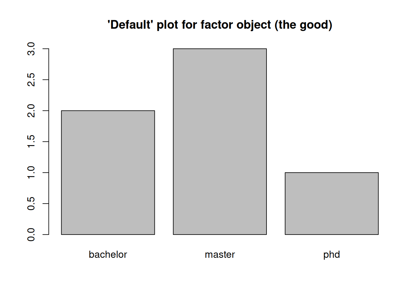

plot(degree, main = "'Default' plot for factor object (the good)")

The bad

When using the integer sequence, R handles the object as a numeric vector. However, standard arithmetic on categorical data is not meaningful! The arithmetic mean or median (as well as minimum/maximum and quartiles) cannot be interpreted!

print(): Not easy to interpret, we would need a lookup-table to decode the information.
summary(): Standard arithmetic is not very meaningful for categorical data.
plot(): Not meaningful, especially not for larger objects.

print(degree_int)

## [1] 2 2 1 3 2 1

summary(degree_int)

##    Min. 1st Qu.  Median    Mean 3rd Qu.    Max. 
##   1.000   1.250   2.000   1.833   2.000   3.000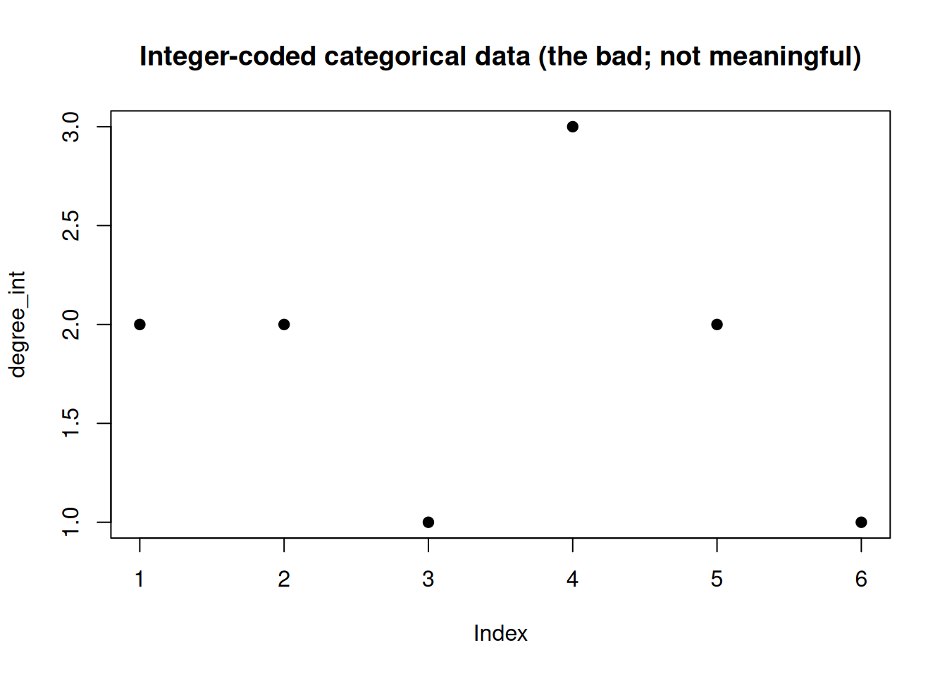

plot(degree_int, pch = 19, main = "Integer-coded categorical data (the bad; not meaningful)")

The ugly

print(): Easy to read, except that we don’t see which categories exist. Otherwise, similar to the output of the factor.
summary(): Does not give us meaningful information.
plot(): Would throw an error, we cannot plot a character vector.

print(degree_chr)

## [1] "master"   "master"   "bachelor" "phd"      "master"   "bachelor"

summary(degree_chr)

##    Length     Class      Mode 
##         6 character character

Computational advantage

In addition, a factor variable has one more advantage. An integer vector of length $N$ requires much less space on your hard drive and in memory, and calculations on integer vectors can be much faster than on character vectors. However, plain integer vectors are less informative (for humans) as readable labels.

Best of both worlds: Factor variables combine the advantages of both; The data are stored as an integer (efficient), the labels have only be stored once as character; while we, as users, still have the advantage of human-readable labels/categories.

11.2 Object orientation

This strategy that we have discussed above for factors can also be applied more generally:

Definition of a suitable class for objects that are then required to have a certain structure.
Providing methods to generic functions for capturing typical computations or workflows based on these objects.
Possibility of organizing classes in a hierarchy so that a child class inherits the behavior from the parent class.

This strategy is sometimes also referred to as object orientation or object-oriented programming (OOP) in the R ecosystem. However, a caveat is that the way this object orientation is implemented in base R is rather different and much more informal compared to other object-oriented languages like C++, Java, or Python. It is also rather different from OOP definitions and discussions in standard computer science textbooks.

This is also the reason that R in fact comes with several object orientation systems, including some that are closer to more standard OOP implementations:

S3: This is the first and simplest object orientation system in R. It is based on generic functions for classes like the factors introduced above.
S4: A somewhat more formal approach, also based on generic functions, but with stricter validity checks of the objects.
Reference classes (RC): More formal OOP implementation where methods belong to the classes/objects directly (and not to generic functions).
R6: An OOP implementation similar to RC but intended to be more lightweight.

Subsequently, we confine ourselves to the basic S3 system which is used in R’s basic statistics functionality and in most commonly-used packages on CRAN. It is elegant in its minimalism and hence relatively easy to adopt for the creation of new classes and methods. Hence subsequently only S3 is introduced in some more detail before showing how custom classes and methods can be created with it.

S3 generics

S3 is based on so-called generic functions. A generic function is a regular function (see Chapter Functions) with a series of arguments and a call to UseMethod() with the name of the generic function in the instruction-part of the function.

This tells R that there are specific methods for specific objects, depending on the class of the object. Let us have a look to the insides of the generic function summary by calling summary (without brackets; shows the function definition).

summary

## function (object, ...) 
## UseMethod("summary")
## <bytecode: 0x581388235580>
## <environment: namespace:base>

If we ignore the last two lines we basically have the following function:

summary <- function(object, ...) {
    UseMethod("summary")
}

We have seen several times what the summary() function returns, and that the returned data summary depends on the class of the object
(numeric vectors, character vectors, matrices, …) given as the first input argument. The function above is not doing that at all. Instead, this is the generic function.

UseMethod("summary") tells R that there must be other functions – now called methods – for objects of different classes.

Arguments

object (required): The main argument when calling summary(). The class of this object determines the dispatch to methods.
...: An arbitrary number of optional arguments passed on to the methods.
Any method must implement these two arguments (object, ...) but may contain further arguments.

Details

When summary() is applied to an object of class "foo", R tries to call the function summary.foo(). If it does not exists, it will call summary.default().
R objects can also have a vector of classes, e.g., c("matrix", "array"), meaning that the object is of class "matrix" inheriting from "array" ("matrix" is a special version of the more generic "array").
In this case, R first tries to apply summary.matrix(), then (if not existing) summary.array(), and then (if both do not exist) summary.default().

Using methods

Methods defined for a certain generic function can be queried using methods().
methods(summary) returns a (long) list of all methods available including summary.factor() and summary.default() (but not summary.numeric(), as summary.default() would be applied to objects of class numeric).
As it is not recommended to call methods directly, some methods are marked as being non-visible to the user and these cannot (easily) be called directly.
Even if visible, it is preferred to call the generic, i.e., summary(g) instead of summary.factor(g)!

Typical generic functions

print(), plot(), summary(), str(), which print, plot, summarize, and describe the structure of an object are available for many classes.
For data classes often: [, [<-, c() (for subsetting and combining objects), coercion functions as.numeric(), as.character() etc. Possibly also format(), mathematical operations etc.
For statistical models (not part of this course; e.g., from lm()): predict(), coef(), residuals(), and many more to do predictions, extract estimated coefficients, or get the residuals of the model.

See what’s defined We can use methods(generic.function, class) to get the available methods for a certain generic function (as above), or a specific class.

Let us see which methods exist for droplevels(). The output below tells us that there is a method for data frames (droplevels.data.frame) and one for factors (droplevel.factor) as shown previously.

methods(generic.function = "droplevels")

## [1] droplevels.data.frame droplevels.factor    
## see '?methods' for accessing help and source code

We might also be interested in what methods exist for an object of a specific class, here class "factor":

methods(class = "factor")

##  [1] [             [[            [[<-          [<-           all.equal    
##  [6] Arith         as.character  as.data.frame as.Date       as.list      
## [11] as.logical    as.POSIXlt    as.vector     c             cbind2       
## [16] coerce        Compare       droplevels    format        initialize   
## [21] is.na<-       kronecker     length<-      levels<-      Logic        
## [26] Math          Ops           plot          print         rbind2       
## [31] relevel       relist        rep           show          slotsFromS3  
## [36] summary       Summary       xtfrm        
## see '?methods' for accessing help and source code

Besides plot(), summary(), and droplevel() we can also see that there is a generic function relevel() which we already used earlier.

Source code: We can always look into the definition of the S3 methods using getS3method(f, class) (f: function name, class: class name).

getS3method("droplevels", "factor")

## function (x, exclude = if (anyNA(levels(x))) NULL else NA, ...) 
## factor(x, exclude = exclude)
## <bytecode: 0x5813911fdac8>
## <environment: namespace:base>

If exported (not all methods are exported) we can get the same result by typing droplevels.factor (no brackets at the end).

Note: Not all methods are implemented for every possible object. Nor are all functions generic. Just as an example, there is no method to combine factor variables (c(a, b) where a and b are factors). Which does not mean we can not implement it ourself! The exercise below tries to demonstrate that.

Combining factors If we simply try c() we will end up with a messed up result as R only combines the two underlying integer vectors.

degree  <- factor(c("master", "bachelor", "bachelor"))
degree2 <- factor(c("phd", "bachelor", "bachelor", "phd"))
c(degree, degree2) # Losing information!!

## [1] master   bachelor bachelor phd      bachelor bachelor phd     
## Levels: bachelor master phd

We could, however, do this manually by:

Coercing both factor objects (degree and degree2) to character.
Combine the two character vectors.
Create a new factor out of it.

This would look as follows:

factor(c(as.character(degree), as.character(degree2)))

## [1] master   bachelor bachelor phd      bachelor bachelor phd     
## Levels: bachelor master phd

Exercise: Instead, we could write a method for that. c() is a generic function, thus we can write a custom c.factor() method ourselves.

Write a function c.factor() (method) with two input arguments.
Internally, create a new combined factor object.
Return the new object.
Test c(degree, degree2) with the two objects above.

Solution. All we need to do is the following:

c.factor <- function(x, y) {
    return(factor(c(as.character(x), as.character(y))))
}
c(degree, degree2)

## [1] master   bachelor bachelor phd      bachelor bachelor phd     
## Levels: bachelor master phd

Et voila, we have a dedicated method to combine factor objects. c(degree, degree2) returns an object of class factor combining both input arguments. And yes, the function above might need some improvements (just for illustration). This is the basic idea of S3 and makes our life easier.

Generalization: The simple demo method (c.factor) above only works for $2$ inputs. We could generalize the function such that it works with $\ne 2$ arguments.

Note that this is way beyond what you need to know, but we can write our c.factor more generic. This uses a series of functions you have not seen (and you don’t have to know)!

# Takes '...' (a list of 1, 2, or N objects),
# converts the content to character and creates
# a new combined factor object.
c.factor <- function(...) {
    return(factor(unlist(lapply(list(...), as.character))))
}
c(degree, degree2) # would also work with 3 or more arguments

## [1] master   bachelor bachelor phd      bachelor bachelor phd     
## Levels: bachelor master phd

11.3 Creating a custom class

So far we have seen how existing classes work – but we can also create our own ones! As motivation: We will use this to handle the air pollution (Luftverschmutzung) data set of Beijing, China. Some big Chinese cities are known for very bad air pollution which can cause serious health issues. We would like to write a class which tells us how often a specific limit (or threshold) was exceeded.

Goal: We will implement a new class called threshold for handling numeric values in combination with a specific limit. Our object should have the following properties, attributes, and methods:

Object properties:
- Type: double (numeric values).
- Length: any length (vectors of length $\ge 1$).
Object attributes:
- Class: threshold.
- limit: single numeric value; our predefined limit.
Methods:
- as.character()/print(): Custom as.character and print methods for now.

As there is no formal definition for S3, all we have to do is to assign a new class to the object pm25, and the threshold we want to use.

pm25 <- c(100, 75, 230, 220, 50)   # Vector for testing
attr(pm25, "limit") <- 150         # Adding attribute 'limit'
class(pm25) <- "threshold"         # Adding class attribute
print(pm25)

## [1] 100  75 230 220  50
## attr(,"limit")
## [1] 150
## attr(,"class")
## [1] "threshold"

We can now write our custom methods with the naming convention genericFunction.className(), e.g., the method for the generic function as.character() must be called as.character.threshold(). The methods should have the same inputs as the generic function; checking by calling as.character (without brackets):

as.character

## function (x, ...)  .Primitive("as.character")

as.character() expects two inputs: x (main object) and ... (further arguments; unused in our case). Our as.character.threshold() should return "+" if a value is above the limit, and "-" else.

as.character.threshold <- function(x, ...) {
    res <- ifelse(x > attr(x, "limit"), "+", "-")
    return(res)
}
as.character(pm25)    # Testing

## [1] "-" "-" "+" "+" "-"

Perfect. Next, we will write the method for print() which re-uses the as.character() method. The first input is x (see generic function print), ... will be unused again.

print.threshold <- function(x, ...) {
    res <- format(x, justify = "right")  # Proper formatting
    res <- paste0(res, as.character(x))  # Combine 'res' with as.character(x)!!
    print(res, quote = FALSE)            # The print we'll see
    invisible(x)                         # Invisible return of the original object
}
print(pm25)

## [1] 100-  75- 230+ 220+  50-

We now have a very specific and easy-to-understand output of our new object class.

Note: This way (see below) it is easy to create objects of the correct class, but with very weird content. Here we have a character vector for our values (instead of numeric values), the limit is not a single numeric value, and the print() method fails (at least throws warnings).

y <- c("foo", "bar")
class(y)         <- "threshold"
attr(y, "limit") <- c(1, 2, 3)
print(y)

## Warning in x > attr(x, "limit"): longer object length is not a multiple of
## shorter object length

## [1] foo+ bar+ foo+

Class constructor function

Much better: Create a class constructor function. This constructor (or initialization) function takes care that the objects are set up properly and only contain what they are allowed to do by providing sanity checking and intelligible error messages.

We have seen a variety of them: factor(), matrix(), vector(), list(), to create objects of specific classes. As we create an object of class threshold, let us define a class constructor function threshold() with two arguments: x (data) and limit.

threshold <- function(x, limit) {
    # Sanity check using stopifnot (short form of if (! ..) stop()).
    stopifnot(is.numeric(x))
    # 'limit' must be numeric, length one, and larger than 0
    stopifnot(is.numeric(limit), length(limit) == 1L, limit > 0)
    # Create our object
    class(x)         <- "threshold"
    attr(x, "limit") <- limit
    return(x)
}
pm25 <- threshold(c(100, 75, 230, 220, 50), limit = 150)
print(pm25)

## [1] 100-  75- 230+ 220+  50-

This ensures that we get a proper threshold object and will throw an error if we do something wrong.

Additional methods

To add more functionality, we can now add additional methods for our new object. In this example, we would like to have a custom summary method and two methods for plotting the data.

Summary: The summary method should show the numeric summary (as for a numeric vector) and a count how often we are above the threshold (using table() on the character representation of our object). Note: the default arguments to summary() are object and ... (would also work if you call it x).

summary.threshold <- function(object, ...) {
    num <- summary(as.numeric(object))    # Numeric summary
    tab <- table(as.character(object))    # Table of character representation
    # Output _to console_:
    cat("Numeric:\n")
    print(num)
    cat("\nTable:")
    print(tab)
    # Invisible return of both
    invisible(list("numeric" = num, "table" = tab))
}
summary(pm25)

## Numeric:
##    Min. 1st Qu.  Median    Mean 3rd Qu.    Max. 
##      50      75     100     135     220     230 
## 
## Table:
## - + 
## 3 2

Plotting functions: To be able to graphically display the data we would like to have two additional methods plot() and hist(). plot() should be a line plot, hist() shows us a histogram with the distribution of the data. We specify some default arguments used to draw the plots and forward ... to the default plotting functions (plot() and hist()) internally. This allows us to change the look if needed.

plot.threshold <- function(x, pch = NULL, type = "o", ...) {
    # Use character representation if pch = NULL
    # to plot a + or - later on.
    if (is.null(pch)) pch <- as.character(x) 
    # Calling default plot function for numeric vectors
    plot(as.numeric(x), pch = pch, type = type, ...)
    # Adding a horizontal line for the limit
    abline(h = attr(x, "limit"), col = "gray", lty = 2)
    # Invisible return 
    invisible(x)
}
par(mfrow = c(1, 2))                         # Subplot definition
plot(pm25)                                   # Default
plot(pm25, col = 2, main = "Test", cex = 3)  # Custom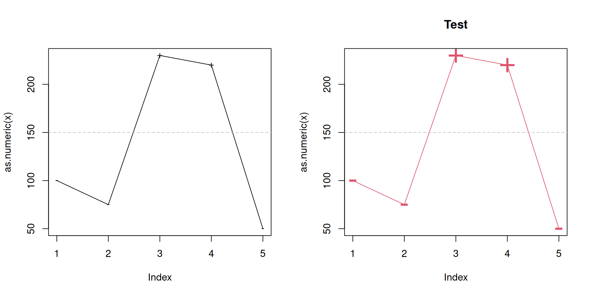

Last but not least we create a similar method for the histogram.

hist.threshold <- function(x, lcol = 2, ...) {
    res <- hist(as.numeric(x), ...)  # Default histogram
    abline(v = attr(x, "limit"), col = lcol, lwd = 2) # Adding limit
    invisible(res) # Return
}
par(mfrow = c(1, 2))                 # Subplot definition
hist(pm25)                           # Default
hist(pm25, lcol = 3, main = "Test")  # Custom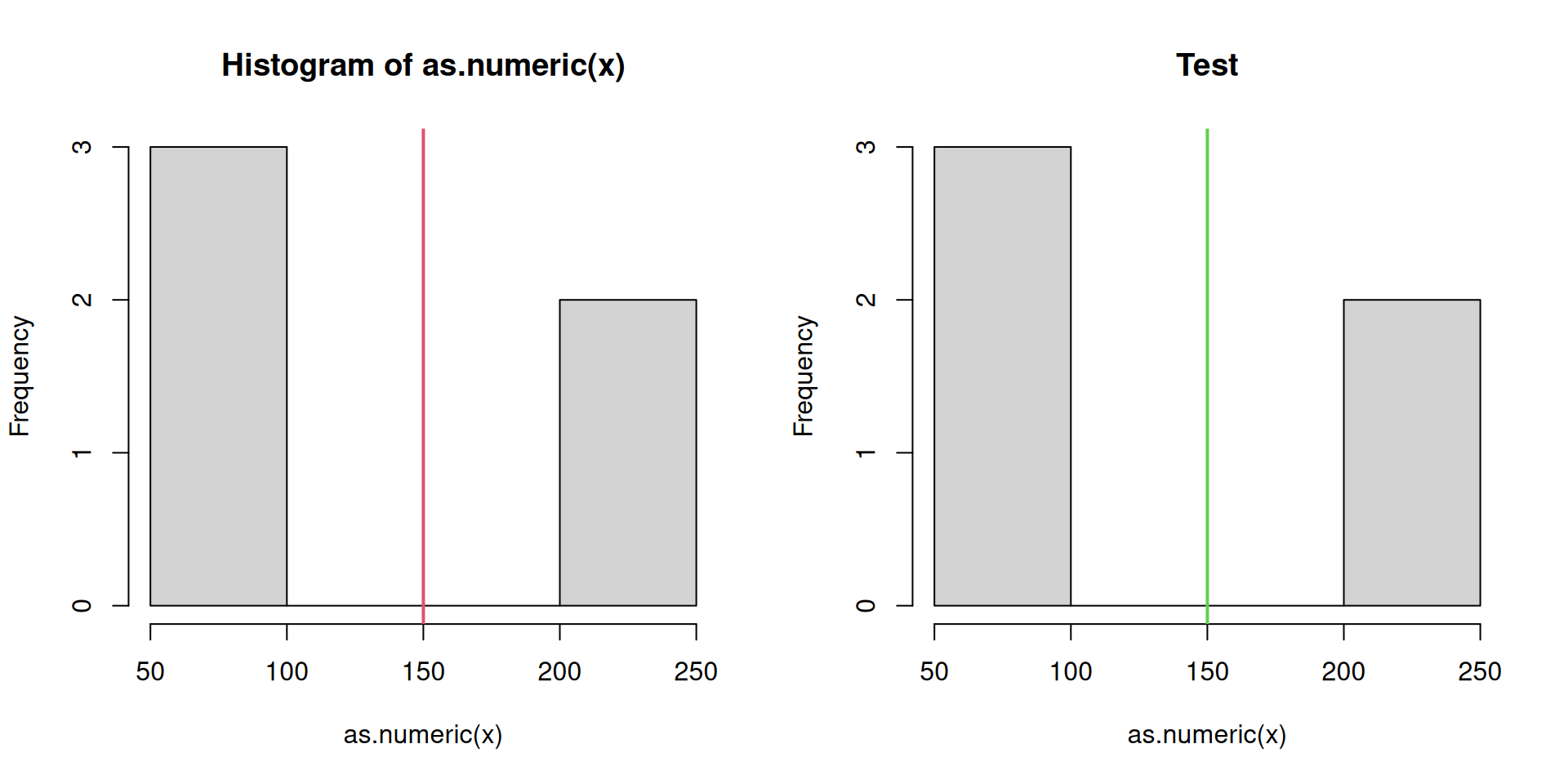

Beijing air quality

Let us now use our new object class for the data set mentioned at the beginning. The data set called “pollution-Beijing.rda” contains air pollution observations for Beijing China from 2015. To be more specific, it contains the daily average PM25 concentration. For short: the lower this value is, the lower the pollution (the better the air quality).

load("data/pollution-Beijing.rda")
plot(pollution$PM25, type = "l", col = 2, main = "PM2.5 Beijing, China, 2015")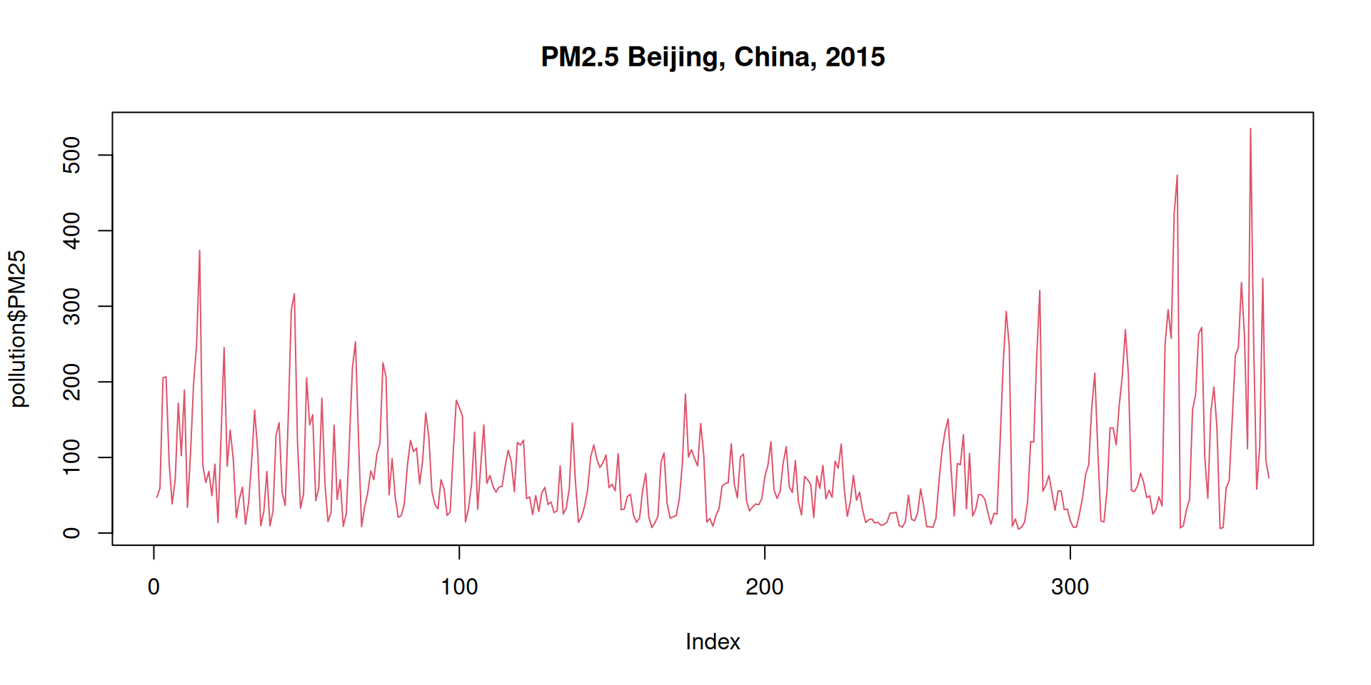

Figure 11.4: Daily mean PM25 concentration in Beijing over entire 2015.

PM25 is the concentration of particles with a diameter of about $2.5$ micrometer, given in micrograms per cubic meter air (particular matter concentration, Feinstaubkonzentration; unit $\mu m m^{-3}$). It is known that these particles can cause serious health issues. Thus, the goal of the European Union was to reduce the annual (yearly) average to less than $25\,\mu m m^{-3}$ in 2015 ($20\,\mu m m^{-3}$ for 2020).

Let us assume that we define a limit of $100$ as the highest allowed concentration and use our custom threshold class to process the data.

Convert pollution$PM25 into an object of class threshold; use limit = 100.
Calculate the summary statistics.
Visualize the data.

load("data/pollution-Beijing.rda")              # Load data
pm25 <- threshold(pollution$PM25, limit = 100)  # Create threshold object
summary(pm25)                                   # Summary

## Numeric:
##    Min. 1st Qu.  Median    Mean 3rd Qu.    Max. 
##    5.10   31.50   60.50   85.86  110.40  535.30 
## 
## Table:
##   -   + 
## 255 110

# Plotting
par(mfrow = c(1, 2))
plot(pm25, main = "Beijing 2015")
hist(pm25, main = "Beijing 2015")

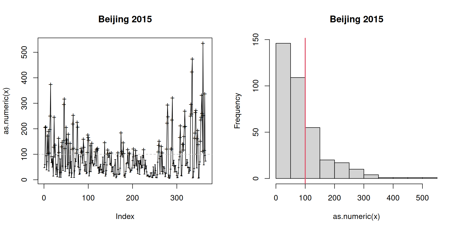
This can be very handy if there is no existing class which can handle your data or you need a more efficient way to handle your own data.

Exercise 11.1 Letters class: As another example to practice, let us create a simple letter class. A class for a single letter (a-z, A-Z).

In this case, we would like to have a new class letter which consists of one single character value.

Class constructor function

Input must be a single character which is in letters (a-z) or LETTERS (A-Z). All other inputs will result in an error.

letter <- function(x) {
    # Sanity checks
    if (!is.character(x)) stop("Input 'x' must be of class character.")
    if (!length(x) == 1L) stop("Input 'x' must be of length 1")
    if (!x %in% letters & !x %in% LETTERS) stop("'x' is no valid letter")
    # Now append class and return the new object
    class(x) <- "letter"
    return(x)
}

# Testing
(x <- letter("A"))

## [1] "A"
## attr(,"class")
## [1] "letter"

(y <- letter(1L))

## Error in letter(1L): Input 'x' must be of class character.

(z <- letter("1"))

## Error in letter("1"): 'x' is no valid letter

Custom print() method

print.letter <- function(x, ...) {
    cat("This is a letter:", dQuote(x), "\n")
    invisible(x)
}
print(x)

## This is a letter: "A"

Summary and structure

In this case, we are happy how the default methods str() and summary() look like, thus we don’t really need to create a custom one. If needed, we could of course write our own str.letter() and summary.letter() methods.

str(letter("A"))

##  'letter' chr "A"

summary(letter("A"))

##    Length     Class      Mode 
##         1    letter character

11.4 Date and date time

We now better understand how different S3 objects are constructed and processed. Let us have a closer look at some other very useful objects: Date and POSIXt. These objects represent dates and date-time and allow for arithmetics (e.g., how many days until new year?).

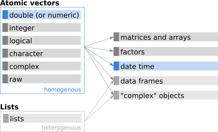
Figure 11.5: Additional base R classes based on atomic vectors.

Technically, a Date or POSIXt object is nothing else than a simple numeric vector, but displayed as a human-readable date (like a string), similar to the factor class.

For both classes a wide range of methods exist which makes it very easy to work with. We’ll only cover few in this chapter. Run the following two commands yourself to see what’s possible.

methods(class = "Date")
methods(class = "POSIXt")

Dates

Calendar dates: Are stored as objects of class Date. No time information.
Structure: Numeric vector; the number of days since 1970-01-01 plus a class attribute.
Creation: Typically from strings (ISO 8301 format; same is used for printing).

(d <- as.Date("2021-01-01"))                       # Default ISO format

## [1] "2021-01-01"

(d2 <- as.Date("29.3.2021", format = "%d.%m.%Y"))  # Custom format

## [1] "2021-03-29"

c(class = class(d), typeof = typeof(d))

##    class   typeof 
##   "Date" "double"

As shown, d is an object of class "Date", type "double", in this case of length 1. If we call unclass(d) all classes are removed which allows us to ‘look inside’ the structure of the object.

unclass(d)

## [1] 18628

As shown, this is all. It’s nothing else than the numeric value $18628$ and a class attribute "Date" (which we just removed here).

Working with dates

The nice thing is that we easily work with this object and e.g., add or subtract integers. E.g.:

Day before d: d - 1.
Date in 7 days from now: d + 7.

The same also works with integer sequences, e.g., seven days starting with d (2021-01-01):

d + 0:6     # 0:6: seven days including 0

## [1] "2021-01-01" "2021-01-02" "2021-01-03" "2021-01-04" "2021-01-05"
## [6] "2021-01-06" "2021-01-07"

Alternatively we can make use of the seq() function to e.g., create a decreasing sequence with a seven-day interval:

seq(from = as.Date("2021-01-01"), 
    to   = as.Date("2020-12-01"),
    by   = -7L)

## [1] "2021-01-01" "2020-12-25" "2020-12-18" "2020-12-11" "2020-12-04"

Multiple date objects can also be used to do some calculations. If we are interested in the number of days between two dates, we simply subtract one from another.

d2 - d

## Time difference of 87 days

as.integer(d2 - d)

## [1] 87

Formatting dates

To format objects of class Date (e.g., for pretty printing or additional processing steps) we can use the generic function format(). This generic is not solely used for for objects of class Date, but many other classes (try methods(generic.function = "format")).

This chapter will only cover the use of the generic function format() for objects of class Date. Let us define a new object birthday as follows:

(birthday <- as.Date("2017-02-01"))

## [1] "2017-02-01"

class(birthday)

## [1] "Date"

format() can now be applied to convert the object into a representation of choice. The function always returns a character vector, wherefore you will lose some functionality (e.g., arithmetics is no longer possible on character representations of a date). However, it can be used for pretty printing or bring your date information into a different format.

When called without any additional arguments, format() will return the date information as an ISO representation. While it looks similar to the original object, it is now of class character.

birthday_pretty <- format(birthday)
print(birthday_pretty)

## [1] "2017-02-01"

class(birthday_pretty)

## [1] "character"

Custom formatting can be defined by providing the additional format argument. The code below, for instance, returns the name of the month or the name of the day from the object birthday:

birthday_month <- format(birthday, format = "%B")
print(birthday_month)

## [1] "Februar"

format(birthday, format = "%A")

## [1] "Mittwoch"

format(birthday, format = "%Y-%m-%d")    # Standard ISO representation

## [1] "2017-02-01"

format(birthday, format = "%d.%m.%Y")    # German date format

## [1] "01.02.2017"

format(birthday, format = "His/her birthday is on %A, %B %d.")

## [1] "His/her birthday is on Mittwoch, Februar 01."

The argument format expects a character which can contain simple text (see above) and/or some formatters like %Y, %m, %d, %B, %A. A few examples are listed in the table below, but many more are available. For a full list of possible formats have a look at the details section of ?strftime.

Note that some of them (e.g., "%B",“%A”`) depend on your system language (not necessarily in English).

Argument	Description	Result
`"%a"`	Abbreviated weekday	`"Wed"`
`"%A"`	Full weekday	`"Wednesday"`
`"%b` or `"%h"`	Abbreviated month	`"Feb"`
`"%B"`	Full month	`"February"`
`"%d"`	Day of the month	`"01"`
`"%j"`	Day of the year	`"032"`
`"%m"`	Month	`"02"`
`"%U"`	Week	`"05"`
`"%x"`	Date	`"02/01/2017"`
`"%Y"`	Year with century	`"2017"`

Time

Note that objects of class Date do not contain any time information. To handle date and time we need objects of class POSIXt. They work the very same as Date objects expect that an increment of +1 is no longer +1 day, but +1 second. This is flagged as additional (optional) content but works the very same as the Date class (including arithmetics or formatting via format()).

Thus, if you are interested in this topic, feel free to read the following ‘excursion’.

Date/time: Stored as objects of class "POSIXct" (inheriting from "POSIXt"); date and time.
Time zone: As dealing with time, the time zone is getting important. If not set, the computer default time zone is used.
Structure: Numeric (double) vector, number of days since 1970-01-01 00:00:00 UTC (“UNIX epoch”), a class attribute, and an additional time zone attribute.
Creation: Typically from strings, defaulting to ISO 8301, also used for printing.

Important to keep in mind: the time zone of your computer is used. The standard time zone of our system (where the book is compiled) uses "UTC" (universal time code). We can explicitly define the time zone using tz = "..." if needed.

(dt1 <- as.POSIXct("2021-01-01 00:00:00"))                # system default is UTC

## [1] "2021-01-01 UTC"

(dt2 <- as.POSIXct("2021-01-01 00:00:00", tz = "CET"))    # Central European time zone

## [1] "2021-01-01 CET"

Checking properties/attributes of dt1:

list(class = class(dt1), typeof = typeof(dt1), attributes = attributes(dt1))

## $class
## [1] "POSIXct" "POSIXt" 
## 
## $typeof
## [1] "double"
## 
## $attributes
## $attributes$class
## [1] "POSIXct" "POSIXt" 
## 
## $attributes$tzone
## [1] ""

As POSIXct inherits from POSIXt we can see that there are two classes (like for matrices c("matrix", "array")). Let us unclass both objects to see how they are constructed:

unclass(dt1)

## [1] 1609459200
## attr(,"tzone")
## [1] ""

unclass(dt2)

## [1] 1609455600
## attr(,"tzone")
## [1] "CET"

As shown, both objects are numeric (double) vectors but contain different numeric values. The numbers always represent the number of seconds to the reference date 1970-01-01 00:00:00 UTC (UTC time zone). As there is one hour offset between “UTC” and “CET”, there is a one-hour difference between these two objects.

dt1 - dt2

## Time difference of 1 hours

As for converting an object of class character to Date, as.POSIXct accepts a custom format definition in case our date and time information (the input) does not come in a standard ISO represesentation.

# From custom format
(d2 <- as.POSIXct("12:47:04, 29.3.2020",
                  format = "%H:%M:%S, %d.%m.%Y"))

## [1] "2020-03-29 12:47:04 UTC"

Working with date/time

As with Date objects we can now work with the POSIXct object(s). Note that, internally, they count the number of seconds. Thus, adding +1 will increase the time by 1 second (not one day as for Date objects).

dt1 - 60                              # 1 minute = 60 seconds

## [1] "2020-12-31 23:59:00 UTC"

dt1 + 3 * 3600                        # 3600 seconds = 1 hour

## [1] "2021-01-01 03:00:00 UTC"

dt1 > dt2

## [1] TRUE

dt1 + 3 * 3600 < dt2

## [1] FALSE

Formatting POSIXt objects

Formatting objects of class POSIXt works in the same way as formatting objects of class Date. Internally, R is now using the dedicated methods format.POSIXct() (or format.POSIXlt(); not covered here) instead of format.Date() as used for objects of class Date. However, the usage is barely different:

format(dt1)

## [1] "2021-01-01"

format(dt1, format = "%Y-%m-%d %H:%M:%S")

## [1] "2021-01-01 00:00:00"

format(dt1, format = "%A %d, %B %Y")

## [1] "Freitag 01, Jänner 2021"

format(dt1, format = "Object `dt1` (%Y-%m-%d %H:%M:%S %Z) belongs to Julian day %j")

## [1] "Object `dt1` (2021-01-01 00:00:00 UTC) belongs to Julian day 001"

format(dt1 - dt2)

## [1] "1 hours"

Or to get a bit more creative (if needed):

format(dt1, "%Hh%mm (on %A %B %d, %Y)")  # Custom formatting

## [1] "00h01m (on Freitag Jänner 01, 2021)"

Plotting

Date and date-time objects are very handy when working with date/time-related data. As an example, let us imagine we have some (random) observations over one year and would like to plot this.

# Generate Date vector over entire 2021
dates <- seq(from = as.Date("2021-01-01"),
             to   = as.Date("2022-01-01") - 1,
             by = 1L)
c(min(dates), max(dates))

## [1] "2021-01-01" "2021-12-31"

# Create some random data -> add both to a data frame.
set.seed(6020) # Pseudo-randomization
df <- data.frame(date = dates, value = rnorm(length(dates)))
head(df)

##         date      value
## 1 2021-01-01 -0.3421647
## 2 2021-01-02  0.4528670
## 3 2021-01-03  0.6169125
## 4 2021-01-04 -0.6121245
## 5 2021-01-05 -1.2603337
## 6 2021-01-06 -0.4266803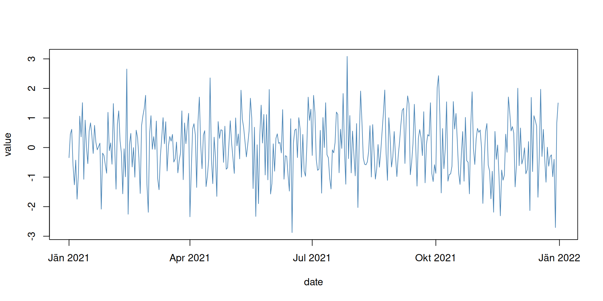

# And plot ...
plot(value ~ date, data = df, type = "l", col = "steelblue")

Or slightly different using type = "h" with different colors for negative/positive values:

plot(value ~ date, data = df, type = "h",
     col = ifelse(value < 0, "steelblue", 2))

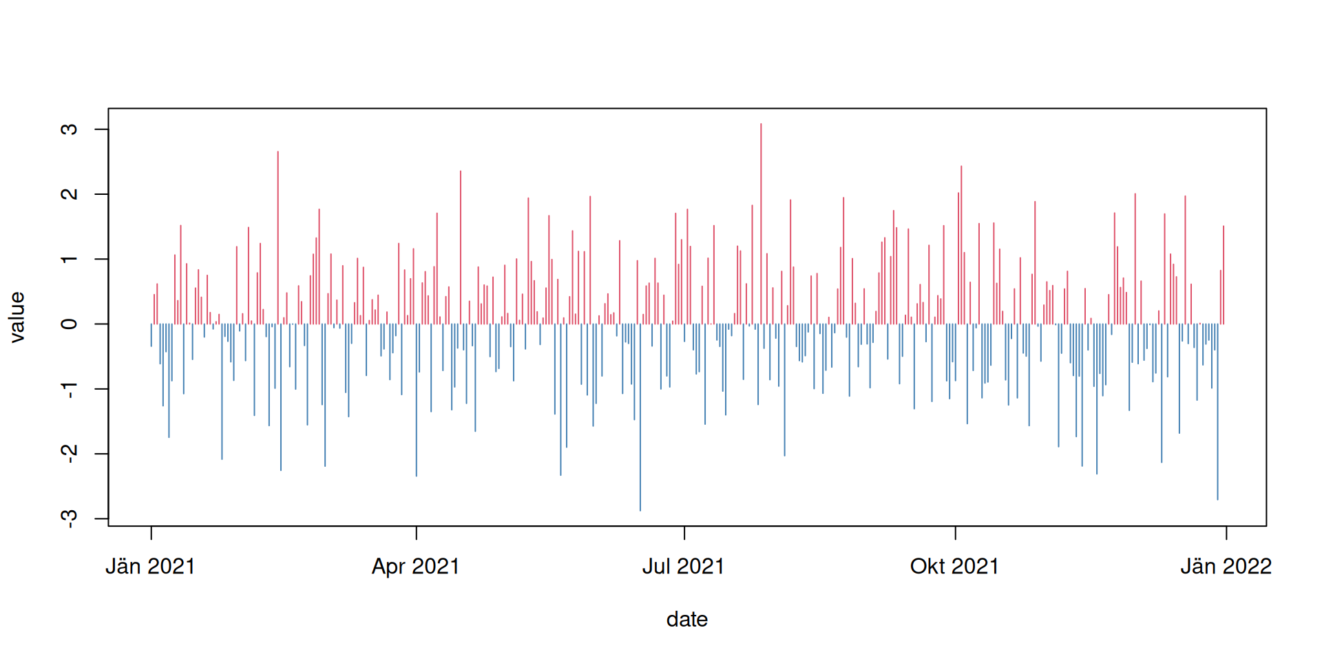
As you can see, R now takes care to plot the data correctly along the x-axis and also adds useful labels. In addition, date and date-time objects are super useful to e.g., calculate annual (yearly), monthly, or daily values (e.g., mean, minimum, maximum) and much more.