Chapter 13 Data Management
Before we start, let us quickly clarify what to expect in this chapter. Data management (how to deal with data sets) and data analysis (explore data, extract information from the data set, draw conclusions) cover a wide range of different topics and can get very complex. The goal of this chapter is to provide an important but relatively basic introduction to data management and some useful functions for exploratory data analysis using data frames in R.
Basic data management
- Screening data sets, data sanity checks and data validation.
- Prepare data for data analysis: Variable transformation, variable/data selection, data aggregation etc.
Basic exploratory data analysis
- Next chapter!
- Descriptive statistics.
- Graphics.
For those who interested in learning more about these topics: the Digital Science Center and other departments of the Universität Innsbruck offer dedicated courses for “Data Management” and “Data Analysis” (as a particular instance, see Data Analytics on discdown.org).
13.1 General strategy
Before going into details, let us define a general strategy how to deal with data. This strategy is not specific to R and can be transferred to other programming languages or programs whenever dealing with (new) data sets.
Typical procedure/steps
- Importing data: Download and import data sets (see Chapter Reading & Writing).
- Data sanity checks:
- Is the structure of the data set OK?
- Initial class/type, dimension, …, for all variables.
- Are there any missing or unrealistic values?
- Use meta-information and data set description if available. Often contain useful information about the data, gaps, units, missing values, …
- Preparation:
- Rename variables and levels.
- Transform variables, factors/classes, unit conversions, combine information, …
- Subset of variables and/or observations of interest.
- Exploratory analysis:
- Descriptive statistics and visualizations.
- Possibly aggregated within subgroups.
- If necessary: Iterate the steps above and adjust your code for preparing the data set.
Now – not earlier – we can start with the formal analysis of the data set, test our hypothesis, set up and estimate our regression models or whatever needed.
Why is this procedure so important?
- Never trust a data set and use it “as it is” without thinking about it and check data at hand.
- The quality of the data set is essential. If you don’t understand the data set, or the data set is simply incorrect/corrupted, your results may be complete rubbish. Or even worse: wrong, but not obviously wrong.
- Helps to avoid wasting time. Nothing is more frustrating than spending days on developing scripts and functions just to find out that “the data set does not provide enough information to answer my (research) question” or “my results are useless as the data set is corrupt/incomplete/wrong”.
13.2 Useful functions
The table below shows a series of functions for the different steps when dealing with ‘data management’ and ‘data analysis’. As you should be familiar to most of them from the previous chapters, we will concentrate on the ones listed under preparation in the following table. The rest of the table can be seen as a recap of useful functions dealing with data and exploratory data analysis.
| Task | Function | Description |
|---|---|---|
| Structure checks |
class()
|
class of object/variable |
typeof()
|
type of object/variable | |
str()
|
structure of an object | |
dim()
|
dimension of rectangular objects | |
head()
|
first \(n\) entries | |
tail()
|
last \(n\) entries | |
names()
|
names/variable names | |
names(x)[3] <- foo
|
replace a specific (variable) name | |
levels(), nlevels()
|
checking factor levels | |
...
|
||
| Data checks |
summary()
|
numerical summary |
plot()
|
generic X-Y plot (and other plot types) | |
is.na()
|
check for missing values | |
duplicated()
|
return duplicated elements/rows | |
anyDuplicated()
|
returns \(\ne 0\) if duplicates are found, \(0\) else | |
unique()
|
get unique elements/rows | |
min()
|
get lowest value | |
max()
|
get highest value | |
range()
|
vector with minimum and maximum | |
...
|
||
| Preparation |
transform()
|
transform a data frame (add, remove, modify variables) |
aggregate()
|
aggregating data | |
reshape()
|
reshape data frames (long form/wide form) | |
x[order(...), ]
|
sort/order the observations of x
|
|
subset()
|
subsetting observations and/or variables | |
...
|
Also
- Try to plan the data management part of your project/task.
- Adhere to good practices: Keep your code with comments etc., such that you can always reproduce the steps taken and check/fix/extend your code.
- When processing different data sets (files) with same format: consider to write a function which imports and prepares the data set.
Disclaimer
- In this chapter we will focus on ‘data management with
data.frameobjects’ only. - For generic functions – such as
transform(),subset(),aggregate()– we will mainly discuss the respectivedata.framemethods. - The goal is an intelligible workflow with base R, e.g., efficiency is not discussed and additional packages are avoided (see next item).
- A series of popular frameworks exist which go beyond base R. For some of
your future tasks they might be required as they offer additional
functionality or are more efficient (memory usage, efficiency). Examples of
commonly used packages are
data.tableanddplyr.
Additional packages such as data.table
or dplyr might get important
once you have very large data sets where they easily outperform the
base R functions. This, however, adds additional dependencies (additional
packages are required to run your code/program).
Especially when using dplyr
(part of Tidyverse) this introduces new objects.
dplyr functions no longer return objects of class data.frame but ‘data frame alike objects’.
While mostly similar to base R data frames not all commands work the very
same and you might need to adjust/rewrite your functions and scripts. Once you
switch to dplyr it makes sense to
use the entire Tidyverse framework which requires
to read/learn how it works.
For those interested, feel free to have a look at the websites for
dplyr and
tidyverse (general information/overview).
Note: Depending on a specific task one has to evaluate whether or not it is beneficial to stick to base R or use additional packages (efficiency, dependencies, knowledge, compatibility, …). For this online learning resource we decided to stick to base R (besides few cases).
13.3 Formula interface
Something which is relatively specific to R is the so called formula interface. Formulae are used in a wide range of (generic) functions when dealing with data sets and become very important when doing data analysis (e.g., data clustering, estimating regression models, …).
A formula allows to express a statistical model – or the relationship between
different variables – in a compact symbolic form. A simple example of a formula
is y ~ x (~ is called a tilde).
- How to read: “
ygivenx” or “yexplained byx”. - Variable of interest: The left hand side of
~is our target (y). - Explanatory variable: The right hand side of
~are our explanatory variables or grouping variables (here onlyx).
For demonstration let us use a formula in combination with plot() given a
simulated data set containing three variables y (target), a (numeric),
and b (factor).
# Generate data set
set.seed(6020)
demo <- data.frame(y = c(rnorm(50, 10, 5), rnorm(30, 12, 3)),
                   a = c(runif(50, 0, 1), runif(30, 0.5, 2)),
                   b = as.factor(rep(c("one", "two"), c(50, 30))))
head(demo, n = 3)
## y a b
## 1 8.289177 0.5731291 one
## 2 12.264335 0.2952761 one
## 3 13.084562 0.1958731 oneWe are interested how y and a relate using a graphical representation
of the data. The same for y and b. In other words, we would like to
visualize
ygivena\(\rightarrow\)y ~ aygivenb\(\rightarrow\)y ~ b
par(mfrow = c(1, 2)) # Two plots side-by-side
plot(y ~ a, data = demo, main = "y explained by a", col = ifelse(b == "one", 1, 2))
plot(y ~ b, data = demo, main = "y explained by b", col = "gray80")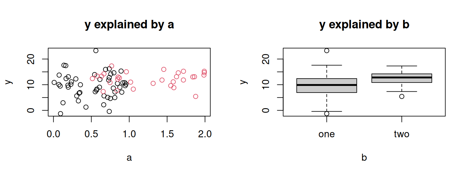
Besides some additional arguments for styling the plots, both commands
are equal (plot(y ~ a), plot(y ~ b)) but yield two different types
of plots. The target (left side of the formula) is plotted on the
y-axis, the variable on the right hand side on the x-axis.
If both are numeric, the result is a scatter plot (left plot), if b
is a character vector or factor, a box-and-whisker plot is getting created.
This is a simple example of how formulae are used, we will come back to
it again later in this chapter. formula is an object class in R and
can be handled like all other objects.
##      class     typeof     length
## "formula" "language" "3"13.4 Toy example
For the upcoming sections where some new functions are introduced, we will use a small toy data set containing six observations of soccer matches. Don’t worry, the data set is easy to understand even for non-soccer enthusiasts. The data set is used to analyze the performance of the team Manchester City (MCI) in the Premier League 2018/2019 against the three other teams that qualified for the Champions League.
(mci <- data.frame(
           team       = rep(c("Liverpool", "Chelsea", "Tottenham"), each = 2),
           type       = rep(c("home", "away"), 3),
           goals      = c(2, 0, 6, 0, 1, 1),
           against    = c(1, 0, 0, 2, 0, 0),
           possession = c(49.6, 49.4, 55.8, NA, 60.7, NA)
        ))
## team type goals against possession
## 1 Liverpool home 2 1 49.6
## 2 Liverpool away 0 0 49.4
## 3 Chelsea home 6 0 55.8
## 4 Chelsea away 0 2 NA
## 5 Tottenham home 1 0 60.7
## 6 Tottenham away 1 0 NAThe teams always play two matches: One at their own city (Manchester, "home")
and one in the home town of the opponent team ("away"). The data set contains:
team: The opponent team MCI is playing against.type: Type of match: home match or away match.goals: How many goals MCI scored (against the opponentteam).against: How many the opponent team scored against MCI.possession: Percent of ball possession of MCI (Ballbesitz; unfortunately some data missing).
Dive into
Before learning the new functions in detail, let us dive into the analysis if the toy data set to get an impression where we are heading; no need to understand everything in detail in this section.
First, we are interested if there are missing values in the data set. We would see this in the summary output, but can also solve it programmatically by (i) counting the overall number of missing values or (ii) count the number of missing values per variable.
## [1] 2## team type goals against possession
## 0 0 0 0 2MCI plays against each team twice, one at home (in Manchester) and once in the
city of the opponent. To make sure that we have no duplicated entries (wrong data)
we check if there are any duplicated entries in team/type (the combination).
## [1] 00 indicates that no duplicated entries have been found and we can start
working with this data set. Our toy data set contains goals and against
but not yet the goal difference (who scored more/less) nor the points gained in
the championship. The rules are:
- \(3\) points: If they (MCI) beat the other team (victory).
- \(1\) points: If both score the same (tie).
- \(0\) points: If they (MCI) gets beaten (loss).
Let us add these two new variables using transform(); The first one (diff)
contains the difference in goals scored by both teams, points contains the
points gained in the Championship.
(mci <- transform(mci,
                  diff   = goals - against,
                  points = ifelse(goals < against, 0, ifelse(goals == against, 1, 3))))
## team type goals against possession diff points
## 1 Liverpool home 2 1 49.6 1 3
## 2 Liverpool away 0 0 49.4 0 1
## 3 Chelsea home 6 0 55.8 6 3
## 4 Chelsea away 0 2 NA -2 0
## 5 Tottenham home 1 0 60.7 1 3
## 6 Tottenham away 1 0 NA 1 3We would like to analyze the performance of MCI in terms of points gained
between home matches and away matches. Does the team perform
better in their own city? Let’s see …
##   type   points
## 1 away 1.333333
## 2 home 3.000000
The function returns the average number of “points given type” and
shows that MCI, on average, scored 3
points at home, while only 1.33
points when not playing in their own city.
What about the minimum/maximum of goals and against
given the type of match and the number of points MCI got?
aggregate(cbind(goals, against) ~ type + points,
          data = mci, FUN = function(x) c(min = min(x), max = max(x)))
## type points goals.min goals.max against.min against.max
## 1 away 0 0 0 2 2
## 2 away 1 0 0 0 0
## 3 away 3 1 1 0 0
## 4 home 3 1 6 0 1Maybe we need the data set in a different form having points for the two
types side by side instead of store in rows. We therefore subset
the variables of interest and reshape the data set.
reshape(subset(mci, select = c(team, type, points)), sep = "_",
        direction = "wide", timevar = "type", idvar = "team")
## team points_home points_away
## 1 Liverpool 3 1
## 3 Chelsea 3 0
## 5 Tottenham 3 3This toy example shows that very detailed analyses can be done with only few lines of code. Let us have a look at the functions in more detail.
13.5 Finding duplicates
One step for checking the data set at hand is to check for duplicated
entries. Base R comes with two functions called duplicated() and anyDuplicated().
duplicated(): Returns a logical vector of duplicated entries.anyDuplicated(): Returns \(0\) if there are no duplicated entries, else the index (integer; always of length 1) of the very first duplicated entry.
The two functions serve specific purposes: duplicated() is used to identify
the elements (observations in case of a data frame) containing duplicated entries,
anyDuplicated() just tells us if there are any (at least one) duplicate and is
very handy for conditional execution.
Usage Let us first check the usage of both functions.
## Default S3 method for duplicated
duplicated(x, incomparables = FALSE,
           fromLast = FALSE, nmax = NA, ...)

## Default S3 method for anyDuplicated:
anyDuplicated(x, incomparables = FALSE,
           fromLast = FALSE, ...)
Arguments
x: a vector or a data frame or an array or ‘NULL’.incomparables: a vector of values that cannot be compared.FALSEis a special value, meaning that all values can be compared.fromLast: logical indicating if duplication should be considered from the reverse side.nmax: the maximum number of unique items expected (greater than one).
Example: We use the defaults for incompareables and nmax solely focussing
on x and fromLast. By default (data frame) the entire observations are checked
for duplicates. Thus, when asking for anyDuplicated(mci) we would expect a \(0\)
as no observation is an exact copy of another one.
# Using the return (0 threaded as FALSE)
if (!anyDuplicated(mci)) cat("No duplicated observations found.\n")
## No duplicated observations found.When checking for duplicated entries one has to define where duplicated
are OK and where they are not allowed to occur. In this case: if the data
set is correct, we should never have duplicated in “team/type”.
On the other hand it is likely and OK that MCI scored the same number of
goals against a specific team. Duplicates in “team/goals” are not a problem.
To search for duplicated entries in a subset of all variables, we make use
of subset():
## [1] 0## [1] 6In the second example anyDuplicated() reports that it found at least one
duplicate in observation \(6\).
Take care: there could be more than only one!
To demonstrate the difference between the two functions let us focus on the
variable against (vector).
## [1] 3## [1] FALSE FALSE TRUE FALSE TRUE TRUE## [1] 3 5 6anyDuplicated() found the first duplicate on index \(3\).
duplicated() returns richer information and tells us all elements which are duplicated
(indices c(3L, 5L, 6L)).
The duplicated entries in mci$against are the \(0\)s in the data set. As shown, the
first occurrence (second row) is not considered to be a duplicate; only following
elements showing the same value are marked as duplicated entries. We can change
this behaviour using fromLast = TRUE, in this case the last occurrence is not
considered to be a duplicated entry.
## [1] 2 3 5Keep in mind: The result of duplicated() (logical vector) can be used for
subsetting and extracting specific observations, anyDuplicated() is used for
control structures like sanity checks or value checks. We could use
sum(duplicated(...)) > 0 to do the same check but this can be much slower
on large data sets. anyDuplicated() stops as soon as it finds the first
duplicate, while duplicated() always checks all data.
Exercise 13.1 Exercise: We have learned how to use unique() and duplicated().
Seems that these are closely related. Can we use duplicated() to
find unique values?
We will work with the following vector of (pseudo-) random letters from A-D.
##  [1] "B" "C" "B" "D" "C" "A" "B" "B" "D" "C" "D" "B" "B" "D" "C" "B" "B" "C" "C"
## [20] "C"- Try to make use of
duplicated()to find all unique values. - Sort your unique vector from above and check if it is identical
sort(unique(x)).
Solution. Unique: Straight forward, we directly sort the resulting vector lexicographically for later on. This, obviously, should result in a vector c(“A”, “B”, “C”, “D”).
## [1] "A" "B" "C" "D"Duplicated: We know that duplicated() returns a logical
vector with elements set to TRUE if this element is a duplicate
of an element which already occurred at least once.
This means that duplicated() always returns FALSE if an element
first occurs (or is unique to that point). Thus, we can select
all elements from x where duplicated() == FALSE or !duplicated().
## [1] 4## [1] "B" "C" "D" "A"Perfect, we only have to sort and check if this is identical to the solution shown above:
## [1] TRUEIs sort() needed? Not in the example/solution shown above. But what
happens if we specify fromLast = TRUE?
## [1] "B" "C" "D" "A"## [1] "A" "D" "B" "C"As you can see, this can change the order of the values. But: unique()
has the same argument. Thus:
## [1] TRUE## [1] TRUENote that x[!duplicated(x)] does the same as unique() and is about as
fast, but we should use unique() when looking for unique values and
duplicated() if we are interested in duplicates.
13.6 Transforming data
We have already learned how to replace, remove and add variables/elements in the
two previous chapters Lists and Data frames.
The function transform() is a convenience function to do the same in a slightly
different way.
Usage
The function returns a modified version of the original data set.
Arguments
_data: The object to be transformed (typically a data frame)....: A series of “tag = value” arguments.
Example: As shown above
this allows us to add variables, but also to modify or delete existing ones.
Let us add a new dummy variable which is nothing else than LETTERS[1:6]
and manipulate points by multiplying them by \(100\).
##        team type goals against possession diff points dummy
## 1 Liverpool home     2       1       49.6    1    300     A
## 2 Liverpool away     0       0       49.4    0    100     B
## 3   Chelsea home     6       0       55.8    6    300     C
## 4   Chelsea away     0       2         NA   -2      0     D
## 5 Tottenham home     1       0       60.7    1    300     E
## 6 Tottenham away     1       0         NA    1    300     F
transform() takes the object mci, evaluates all tag = value arguments
(important: tag = value not tag <- value!), appends them to the original object and
returns it. As for subset() we can directly use the variable names (here points)
and do not have to specify mci$points.
If R finds the variable (goals) in the object provided as input, this
variable will be taken for calculation. Note: it is not possible to directly
use newly created variables within one transform() call (dummy
in this case).
Return value: The return is a modified version of the original input mci.
We can also remove existing variables by assigning a NULL to them.
As we have ‘messed up’ the points column, we fix this in the same call.
(mci <- transform(mci,
                  dummy = NULL,              # Delete this variable
                  points = points / 100))    # Fixing 'points'
## team type goals against possession diff points
## 1 Liverpool home 2 1 49.6 1 3
## 2 Liverpool away 0 0 49.4 0 1
## 3 Chelsea home 6 0 55.8 6 3
## 4 Chelsea away 0 2 NA -2 0
## 5 Tottenham home 1 0 60.7 1 3
## 6 Tottenham away 1 0 NA 1 3Job done. We could, of course, do the same without using the function
transform(). Check out the following exercise.
Exercise 13.2 Practical exercise: Instead of using transform() we could
do the same using the $ operator (or subsetting) and assign/modify/delete
variables. Try to start over with the original object mci and do the same
without using transform().
# Start with this object (called mci2 now)
(mci2 <- data.frame(
           team    = rep(c("Liverpool", "Chelsea", "Tottenham"), each = 2),
           type    = rep(c("home", "away"), 3),
           goals   = c(2, 0, 6, 0, 1, 1),
           against = c(1, 0, 0, 2, 0, 0)
        ))
## team type goals against
## 1 Liverpool home 2 1
## 2 Liverpool away 0 0
## 3 Chelsea home 6 0
## 4 Chelsea away 0 2
## 5 Tottenham home 1 0
## 6 Tottenham away 1 0- Add new variable
diffandpoints. - Add new variable
dummycontainingLETTERS[1:6], multiplypointsby a factor of100. - Delete
dummy, correctpoints.
Solution. Starting from this object:
# Start with this ..
(mci2 <- data.frame(
          team    = rep(c("Liverpool", "Chelsea", "Tottenham"), each = 2),
          type    = rep(c("home", "away"), 3),
          goals   = c(2, 0, 6, 0, 1, 1),
          against = c(1, 0, 0, 2, 0, 0)
       ))
## team type goals against
## 1 Liverpool home 2 1
## 2 Liverpool away 0 0
## 3 Chelsea home 6 0
## 4 Chelsea away 0 2
## 5 Tottenham home 1 0
## 6 Tottenham away 1 0Adding two new columns:
mci2$diff   <- mci2$goals - mci2$against
mci2$points <- ifelse(mci2$goals < 0, 0, ifelse(mci2$goals == mci2$against, 1, 3))
head(mci2, n = 2)
## team type goals against diff points
## 1 Liverpool home 2 1 1 3
## 2 Liverpool away 0 0 0 1Add dummy, multiply points:
## team type goals against diff points dummy
## 1 Liverpool home 2 1 1 300 A
## 2 Liverpool away 0 0 0 100 BRemove dummy, correct points:
##        team type goals against diff points
## 1 Liverpool home     2       1    1      3
## 2 Liverpool away     0       0    0      1
## 3 Chelsea home 6 0 6 3
## 4 Chelsea away 0 2 -2 3
## 5 Tottenham home 1 0 1 3
## 6 Tottenham away 1 0 1 3We can also do it this way, but needs more typing than
when using the transform() function and makes the commands harder to read,
especially if you do more complex calculations to create new variables.
Besides transform() two additional functions exist which can become
very handy but will not be discussed further in this chapter.
within(): Similar totransform(); no longer usestag = valuesyntax but takes a series of expressions evaluated in an encapsulated environment (inside the function). Allows to directly use newly created variables if needed.with(): Does not modify the original object; only returns one new variable. Sometimes handy to reduce code complexity.- For both: Check out documentation on
?withor?within(same).
13.7 Aggregating data
A new useful generic function is aggregate() allowing for data aggregation.
You may notice similarities to tapply(), one of the loop replacement
functions, however, aggregate() is no loop replacement function itself.
aggregate() (as it is a generic function) can be applied to objects of
different classes, we will cover use cases in this chapter: Using
the generic S3 function for data.frames and the generic S3 function
for formula (see Formula interface).
Usage: The manual page (see ?aggregate) shows
how to use the function in these two cases (data.frame’s/formula):
## S3 method for class 'data.frame'
aggregate(x, by, FUN, ..., simplify = TRUE, drop = TRUE)

## S3 method for class 'formula'
aggregate(x, data, FUN, ...,
          subset, na.action = na.omit)
In both cases (shown below) we can achieve the same results. However, the default behaviour of the two S3 methods distinctly differ, especially for processing multivariate data.
Usage: S3 method for class ‘formula’ (if the first input is a formula;
see ?aggregate for details).
Arguments for use with data.frame’s:
x: an R object (vector or data.frame).by: a list of grouping elements, each as long as the variables in the data framex. The elements are coerced to factors before use.FUN: a function to compute the summary statistics which can be applied to all data subsets.
Arguments for use with formula:
formula: a formula, such asy ~ xorcbind(y1, y2) ~ x1 + x2, where theyvariables are numeric data to be split into groups according to the groupingxvariables (usually factors).data: a data frame (or list) from which the variables in formula should be taken.FUN: a function to compute the summary statistics which can be applied to all data subsets....: further arguments passed to or used by methods.subset: an optional vector specifying a subset of observations to be used (as insubset()).na.action: a function which indicates what should happen when the data containNAvalues. The default is to ignore missing values in the given variables (Note: will be discussed in detail later).
Example: We are interested in the mean number of points given type of match
(points ~ type; as shown above)
and calculate the mean() based on our data set mci.
##   type   points
## 1 away 1.333333
## 2 home 3.000000
Instead of the arithmetic mean we can also return the range (minimum to
maximum) of the goal differences given type of match or the 0.5 quantile
(\(50\%\) percentile; also known as median) of points given type of match. Note
that probs is forwarded to our function quantile() via the ... argument
of aggregate().
# Range of goal differences
aggregate(diff ~ type,   data = mci, FUN = range)
# .5 quantile: same as FUN = median.
aggregate(points ~ type, data = mci, FUN = quantile, probs = 0.5)
If we would like to aggregate multiple variables at once, the left hand side
(target) of the formula can be extended using cbind() using a comma separated
list of variable names to be aggregated.
##   type     goals   against       diff   points
## 1 away 0.3333333 0.6666667 -0.3333333 1.333333
## 2 home 3.0000000 0.3333333  2.6666667 3.000000
In this case the arithmetic mean is calculated for all four variables on the
left hand side at once, calculating the mean for goals ~ type, against ~ type, diff ~ type and points ~ type. We can also extend the right hand
side of the formula, e.g., aggregating the number of goals given type and points.
##   type points goals.1 goals.2
## 1 away      0       0       0
## 2 away      1       0       0
## 3 away      3       1       1
## 4 home      3       1       6
The combination of type and points are now unique (all possible combinations),
the latter two columns contain minimum/maximum number of goals. When only looking
at the last line of the result we get the information that:
- Whenever MCI played a home match and got \(3\) points (won the match) they scored at least \(1\) up to \(6\) goals.
Exercise 13.3 tapply() versus aggregate(): Just for practicing, use
tapply() instead of aggregate() to get the same information.
We have seen the following command above, aggregating the points
difference given type (home/away).
# Mean point difference given type of match (home or away)
(res_agg <- aggregate(diff ~ type, data = mci, FUN = mean))
## type diff
## 1 away -0.3333333
## 2 home 2.6666667- Use
tapply()to get the same information (mean difference). - Advanced: try to create an object identical to
res_aggusing the result returned bytapply().
Solution. Disclaimer: This exercise is just for practicing purposes,
in reality you would stick to aggregate() which is much more
convenient.
tapply(): We are interested in mci$diff and group by
mci$type; that is what the formula diff ~ type expresses
used when calling aggregate(), and apply the function mean().
##       away       home
## -0.3333333  2.6666667
Make the objects identical: tapply() returns us a named
vector while aggregate() returns a data frame. Furthermore,
the variable names are gone when using tapply().
What we need to do:
- Create a new data frame.
- Take the names of the named vector
res_tapplyand store this information as the first variabletype. - Take the content (mean) and store it as second variable
diff. - Compare the two objects.
## [1] TRUENot good practice as we have hard-coded variable names when creating
the new data frame (data.frame(type = ..., diff = ...)). But as mentioned,
this was just for practicing.
Not using formula interface: It is possible to use aggregate()
not using the formula interface. In case our first input to aggregate()
is not a formula but e.g., a data frame the usage of the function differs.
Usage: Using a data frame as first input (similar to what we have seen for tapply().
x: an R object (data frame in this case).by: a list of grouping elements, each as long as the variables in the data frame ‘x’. The elements are coerced to factors before use.FUN: Out function to be applied.
Example: Let us do the same as above.
##   Group.1     goals   against       diff   points
## 1    away 0.3333333 0.6666667 -0.3333333 1.333333
## 2    home 3.0000000 0.3333333  2.6666667 3.000000
Getting the same information and an object similar to using the formula interface.
Aggregation with missing values
When evaluating functions such as sum() or mean() on data with missing values,
R’s default strategy is to return NA for the result. Alternatively, one often
removes or omits the missing values prior to evaluating the function (typically by
setting na.rm = TRUE).
In principle, the same can be done when aggregating data with missing values. However, the question how to remove missing values becomes more complex when multivariate data is aggregated.
- Conceptually, there are two strategies: The
NAs for all variables can be handled simultaneously, i.e., the entire row of data is omitted when there is at least oneNA(complete cases). Or, alternatively, theNAs can be dealt with per variable (available cases). - In
aggregate(), the defaults for dealing with missing values differ between the default method (available cases) and the fomula method (complete cases). - Both methods can carry out both strategies, though.
As shown above, the variable possession contains 2
missing values. Let us assume to be interested in the average number of goals as
well as the average possession for each type of game (home vs. away) by performing the aggregation
once (i) using the S3 method for data frames (default) and once (ii) using the formula interface.
# (i) Aggregation using the default interface
aggregate(subset(mci, select = c(goals, possession)), list(mci$type), FUN = mean)
## Group.1 goals possession
## 1 away 0.3333333 NA
## 2 home 3.0000000 55.36667# (ii) Using the formula interface
aggregate(cbind(goals, possession) ~ type, data = mci, FUN = mean)## type goals possession
## 1 away 0 49.40000
## 2 home 3 55.36667Both work (no errors, no warnings) but show different results due to the different default behaviour of the two methods.
- Default: uses all available cases for aggregation, thus also using the rows containing missing values.
- Formula: only uses the complete cases, thus removing all observations (rows) which contain at least one missing value before aggregating the data.
The figure below illustrates the difference between the two cases.
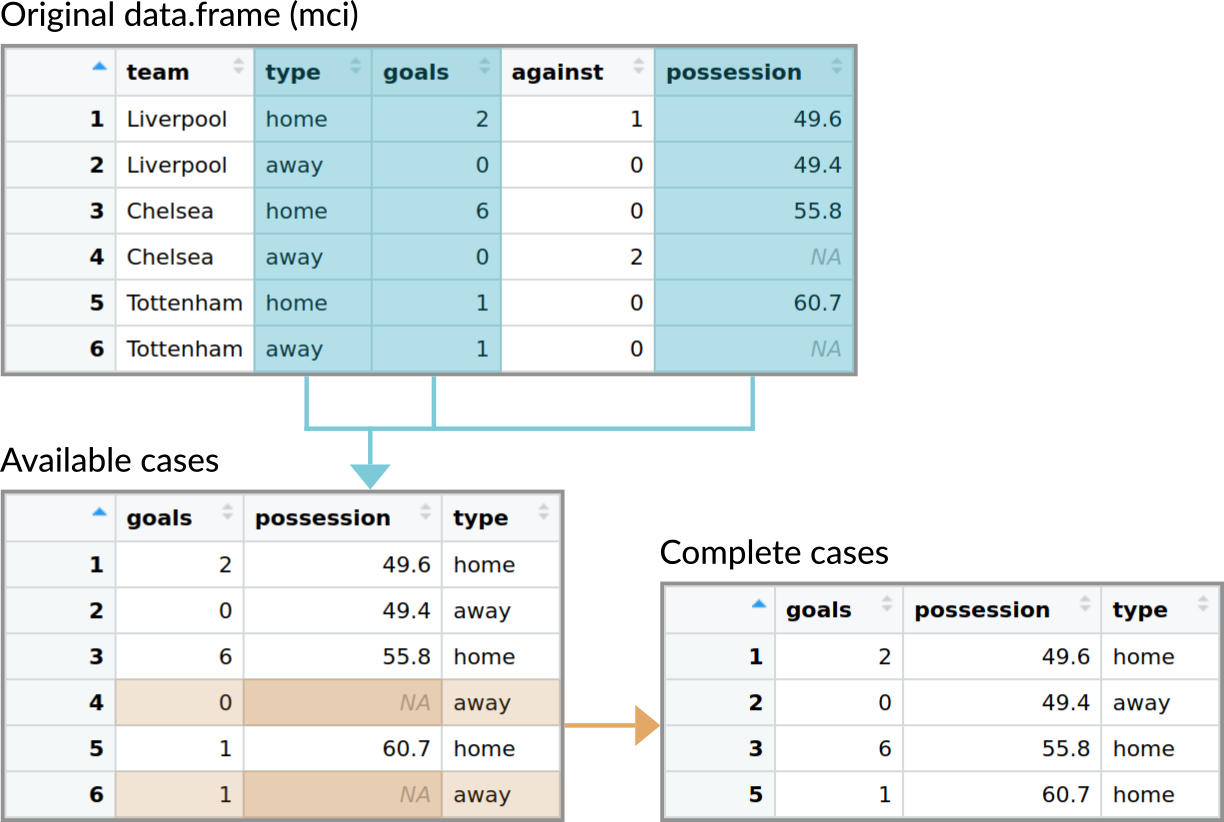
Figure 13.1: Illustration of the data used when aggregating data with either the default method for data.frames (uses available cases by default) and when using the method with a formula (uses complete cases by default).
As shown at the beginning of this section (usage; see also ?aggregate) this is due to the
default argument of the methods. The default method for data frames has no special argument
on how to deal with missing values, the formula method uses na.action = na.omit.
In both cases we can change the behavior if needed. In case of the default method we can
specify the additional argument na.rm = TRUE. As this is none of the argument of the
function itself, it will be forwarded to our FUN. Thus, instead of using mean(...)
it will call mean(..., na.rm = TRUE).
aggregate(subset(mci, select = c(goals, possession)), list(mci$type), FUN = mean,
          na.rm = TRUE) # <- additional argument
## Group.1 goals possession
## 1 away 0.3333333 49.40000
## 2 home 3.0000000 55.36667Note that we no longer have NAs in the aggregated result, however, the average
number of goals differs from the result above as it uses the goals of all matches
(the mean goals are based on 3 values each, for possession it uses 3 values for
type = "home" but only one for type = "away").
When using the formula interface we can specify na.action = na.pass which lets missing
values pass by, in other words using all available cases. This results in the very same
result as when using the default method (without na.rm = TRUE).
##   type     goals possession
## 1 away 0.3333333         NA
## 2 home 3.0000000   55.36667
Thus, be aware of possible missing values when using aggregate to be sure to get the result you want.
13.8 Reshaping data
Re-shaping data from what is called a ‘long format’ to a ‘wide format’
is frequently needed. Base R comes with the function reshape() which
allows to convert a data set from one form into another. Our toy data set
is currently in the long format – let us first have a look at this data
set in long and wide format focussing on team, type and points only.
##        team type points
## 1 Liverpool home      3
## 2 Liverpool away      1
## 3   Chelsea home      3
## 4   Chelsea away      0
## 5 Tottenham home      3
## 6 Tottenham away      3
## team points.home points.away
## 1 Liverpool 3 1
## 3 Chelsea 3 0
## 5 Tottenham 3 3This function is not changing data, but putting it in different shape
(re-shape). Let us define the team as our ‘entity’. In the long format the
‘entity’ (team) can occur multiple times, while in the wide format each
‘entity’ only occurs once while all information is stored in the variables.
Important: In statistics and economics a common format for handling data
are “panel data”
where we typically have observations for a series of entities (e.g., persons, countries)
over time (e.g., happiness over years, gross domestic product over years).
This specific type of information is the motivation behind the function reshape()
provided by base R and the names of its arguments which can make the use of reshape()
somewhat confusing.
We can think about our object mci the same way: we have some entities (team)
and varying information (points). Instead of time (years) the information
varies with the type of match. type is the attribute which links the entity team
to the varying information.
Note: Won’t be used extensively in this book/our course, but keep in mind this exists as it might become very handy when working with data sets in the future which often come in the ‘long format’, while we might need the ‘wide’ format to analyze the data.
Example: Our mci data set is currently in a long format. To get to the
wide format (as sown above) we can call the following command:
(mci_wide <- reshape(mci,
                     direction = "wide",     # Reshape to 'wide'
                     v.names   = "points",   # Varying variables/variables of interest
                     idvar     = "team",     # Grouping (in rows)
                     timevar   = "type",     # Grouping (in columns)
                     drop      = c("possession", "diff", "goals", "against"))) # Drop them
## team points.home points.away
## 1 Liverpool 3 1
## 3 Chelsea 3 0
## 5 Tottenham 3 3The data set is re-shaped to the wide format. idvar defines the variable
containing the entity (team) and timevar the attribute which connects the
entity to the data in v.names. This also works from wide to long, however,
rather complicated.
Instead: Let us have a look at two functions from an additional package
called tidyr which might be
easier to understand. The package provides two functions called:
pivot_longer(): converts wide to long.pivot_wider(): converts long to wide.
Let us use the object mci once again and convert it to wide and back.
Again, only team, type, goals and diff will be used for simplicity.
library("tidyr")  # Might need to be installed once

(mci_wide <- pivot_wider(subset(mci, select = c(team, type, points)),
                         names_from = "type", values_from = "points"))
## # A tibble: 3 × 3
## team home away
## <chr> <dbl> <dbl>
## 1 Liverpool 3 1
## 2 Chelsea 3 0
## 3 Tottenham 3 3What we get as a result is a ‘tibble data frame’ as
tidyr
is part of Tidyverse which could be
converted to a pure data frame using as.data.frame() if needed. Let us now
take the mci_wide and re-shape back to a long format.
## # A tibble: 6 × 3
##   team      type  points
##   <chr>     <chr>  <dbl>
## 1 Liverpool home       3
## 2 Liverpool away       1
## 3 Chelsea   home       3
## 4 Chelsea   away       0
## 5 Tottenham home       3
## 6 Tottenham away       3
What we can see is that we do not have the same object as before.
This data set only contains three variables, namely team (entity),
type (attribute) and points (value) which is known as the
entity-attribute-value model.
Once more: Keep this in mind but don’t worry, will not be used intensively for the rest of this book.
13.9 Subsetting data
We have already learned how the function subset() works in
Subchapter ‘Subsetting data frames’.
For the sake of completeness:
Usage
Arguments
x: object to be subsetted.subset: logical expression indicating elements or rows to keep; subsetting observations/rows.select: expression, indicating columns to select from a data frame; subsetting variables/columns.drop: passed on to ‘[’ indexing operator; allows to drop data frame attributes if only one variable is returned (to get a vector).
Examples
##      team type goals
## 3 Chelsea home 6## [1] 0 6 1 113.10 Sorting & Ordering
One step of preparing our data set is to sort (change the order) of the
observations. There is no dedicated function to sort() a data frame.
Instead we make use of order() in combination with subsetting by index.
Usage
Important arguments
...: a sequence of numeric, complex, character or logical vectors, all of the same length.decreasing: logical. Should the sort order be increasing or decreasing?na.last: for controlling the treatment of ’NA’s.
Examples
Order/sort by one variable against, decreasing (lexicographically).
##        team type goals against possession diff points
## 4   Chelsea away     0       2         NA   -2      0
## 1 Liverpool home     2       1       49.6    1      3
## 2 Liverpool away     0       0       49.4    0      1
## 3   Chelsea home     6       0       55.8    6      3
## 5 Tottenham home     1       0       60.7    1      3
## 6 Tottenham away     1       0         NA    1      3
Order/sort by two variables type and goals; increasing (default).
First the data set is sorted by type. If a specific value in type
occurs more than once, the second variable (goals) is used to sort
the observations given this type.
##        team type goals against possession diff points
## 2 Liverpool away     0       0       49.4    0      1
## 4   Chelsea away     0       2         NA   -2      0
## 6 Tottenham away     1       0         NA    1      3
## 5 Tottenham home     1       0       60.7    1      3
## 1 Liverpool home     2       1       49.6    1      3
## 3   Chelsea home     6       0       55.8    6      3
13.11 Real world example
After introducing a general strategy how to import, check, transform, and aggregate data based on a very simple toy data set let us apply these steps on a larger real world data set. In this last section we will use an XLSX file “cod.xlsx” (click to download) from Zuur et al. (2009) originally taken by Hemmingsen et al. (2005; Marine Pollution Bulletin).
The data set was used to investigate the distribution of a specific blood parasite in Cods (Kabeljau). This parasite transmitted via Leeches (Blutegel) which like to lay their eggs on the carapace (Panzer/Schale) of the red king crab (rote Königskrabbe) which has been put into the Barents Sea in the 1960s by the Russians to serve as a resource of food.
.](images/13/13-paper-hemmingsen.png)
Figure 13.2: Figure 1 and 2b from the original publication Hemmingsen et al. 2005.
The hypothesis
- The more crabs, the more the Leech reproduce.
- The more Leech, the more the parasite is transmitted to the Cods.
Data set information
- XLSX (Excel) file format (cod.xlsx).
- Contains 1254 observations; 1254 Cods fished.
- intensity: Intensity of parasite infection.
- prevalence: Boolean value; parasite present?
- area/year/depth: Where and when the Cod was caught.
- weight/length/sex/age: Information about the fish.
- stage: Stage of the leech (life-cycle; the leech must leave the fish host at a later stage and lay its eggs).
(1) Importing the data set
First we need to import the data set using readxl in this case
and investigate the returned object.
read_excel() returns a ‘tibble data frame’ which we can easily
convert to a base R data frame (not necessary).
##   intensity prevalence     area year depth weight length sex stage age
## 1         0          0 mageroya 1999   220    148     26   0     0   0
## 2         0          0 mageroya 1999   220    144     26   0     0   0
## 3         0          0 mageroya 1999   220    146     27   0     0   0
(2) Data sanity checks
Once imported we can perform data sanity checks. Is the structure of the object OK? Do we have missing values? Are all values valid and meaningful?
## 'data.frame':    1254 obs. of  10 variables:
##  $ intensity : num  0 0 0 0 0 0 0 0 0 0 ...
##  $ prevalence: num  0 0 0 0 0 0 0 0 0 0 ...
##  $ area      : chr  "mageroya" "mageroya" "mageroya" "mageroya" ...
##  $ year      : num  1999 1999 1999 1999 1999 ...
##  $ depth     : num  220 220 220 220 220 220 220 194 194 194 ...
##  $ weight    : num  148 144 146 138 40 ...
##  $ length    : num  26 26 27 26 17 20 19 77 67 60 ...
##  $ sex       : num  0 0 0 0 0 0 0 0 0 0 ...
##  $ stage     : num  0 0 0 0 0 0 0 0 0 0 ...
##  $ age       : num  0 0 0 0 0 0 0 0 0 0 ...
What we get is a data frame with 1254 observations and 10
variables whereof 9 are numeric and
1 character.
To check the range of the values (minimum/maximum) and the number of missing
values we have a look at summary().
##    intensity         prevalence         area                year
##  Min.   :  0.000   Min.   :0.0000   Length:1254        Min.   :1999
##  1st Qu.:  0.000   1st Qu.:0.0000   Class :character   1st Qu.:1999
##  Median :  0.000   Median :0.0000   Mode  :character   Median :2000
##  Mean   :  6.183   Mean   :0.4536                      Mean   :2000
##  3rd Qu.:  4.000   3rd Qu.:1.0000                      3rd Qu.:2001
##  Max.   :257.000   Max.   :1.0000                      Max.   :2001
##  NA's   :57        NA's   :57
##      depth           weight           length            sex
##  Min.   : 50.0   Min.   :  34.0   Min.   : 17.00   Min.   :0.000
##  1st Qu.:110.0   1st Qu.: 765.5   1st Qu.: 44.00   1st Qu.:1.000
##  Median :180.0   Median :1432.0   Median : 54.00   Median :1.000
##  Mean   :176.2   Mean   :1704.3   Mean   : 53.45   Mean   :1.411
##  3rd Qu.:235.0   3rd Qu.:2222.5   3rd Qu.: 62.00   3rd Qu.:2.000
##  Max.   :293.0   Max.   :9990.0   Max.   :101.00   Max.   :2.000
##                  NA's   :6        NA's   :6
##      stage            age
##  Min.   :0.000   Min.   : 0.00
##  1st Qu.:1.000   1st Qu.: 3.00
##  Median :1.000   Median : 4.00
##  Mean   :1.409   Mean   : 4.07
##  3rd Qu.:2.000   3rd Qu.: 5.00
##  Max.   :4.000   Max.   :10.00
## - We have some missing values in intensity, prevalence, weight, length.
weight: Maximum of 9990; is this realistic?sex: Seems we have three values forsex(0 is wrong).age: 84 fishes have age \(0\). Most likely as the age is rounded; thus OK.prevalence: seems to be eitherTRUE(1) orFALSE(0).- Some variables (
sex,area) are categorical data and should be transformed to factor.
Exercise 13.4 Start an R session yourself and try to look into these things in detail.
- Programmatically get number of observations/variables, and class of all variables.
- Programmatically extract the names of the variables which contain missing values.
- Get the maximum of
weight. Plot the vectorweight. Is 9990 the only obviously wrong one? - Check unique values of
sex. Count how often each of these values occurs in the data set. - Plot (
hist()) the variableage. In addition, count how often age \(0\) occurs in the data set.
Solution. Number of observations/variables, class of all variables
The first one is simple:
n_obs  <- nrow(cod)
n_vars <- ncol(cod)
cat("We have", n_obs, "observations and", n_vars, "variables.\n")
## We have 1254 observations and 10 variables.To get the class of each of the variables we could make use of sapply().
## cod_classes
## character   numeric
##         1         9
Extract the names of the variables containing NA
We can count missing values in a vector using sum(is.na(x)). To apply
this function to each variable individually, we again make use of sapply().
##  intensity prevalence       area       year      depth     weight     length
##         57         57          0          0          0          6          6
##        sex      stage        age
##          0          0          0
Using a relational operator to find the elements where we have at least one
missing value (we could also use != 0 instead of > 0) and use this logical
vector to get the names we need.
## [1] "intensity" "prevalence" "weight" "length"Get the maximum of weight
To get the maximum we have to take care that we have missing values in this variable.
## Maximum weight is 9990 .Let us plot the weight to see if this value is meaningful or an outlier.
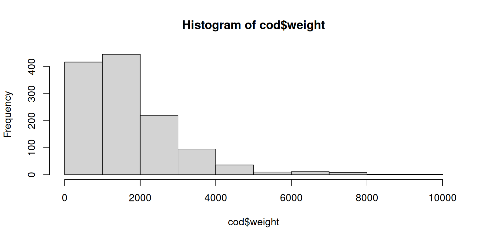
While most fishes weight below \(2000\), 9990 does not seem to be an outlier, but a decently heavy fish. Given this plot the values do look meaningful.
Check unique values of sex
Using unique() to find all unique values, or directly use table() which gives
us both, all unique values and absolute counts (how often each one occurs).
##
##   0   1   2
##  82 574 598
Plot (hist()) the variable age
Count number of fished being of age \(0\) and plot the distribution of age.
We use the number of fishes being \(0\) in the title.
n_zero <- sum(cod$age == 0, na.rm = TRUE)
hist(cod$age, main = paste("Age of fish,", n_zero, "of age 0"))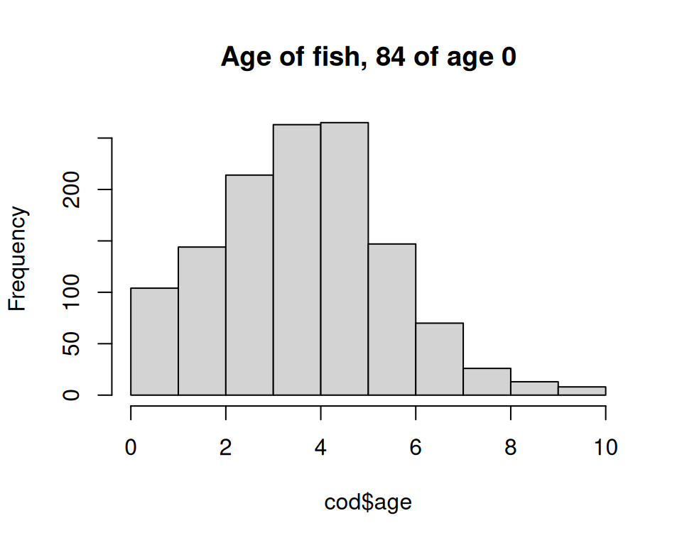
(3) Preparation
Once we have identified problems we can now prepare our data set.
- Rename variables: Not required in this case (except you prefer to do so).
- Transform variables: We would like to transform some into
factor/logical. - Subset: Subset the data set to remove data we don’t need (e.g., missing values,
or
sex == 0).
Transforming variables
We can use transform() to transform the three variables prevalence, area
and sex all in one go.
cod <- transform(cod,
               prevalence = as.logical(prevalence),
               area       = as.factor(area),
               sex        = factor(sex, 1:2, c("male", "female")))
str(cod)
## 'data.frame': 1254 obs. of 10 variables:
## $ intensity : num 0 0 0 0 0 0 0 0 0 0 ...
## $ prevalence: logi FALSE FALSE FALSE FALSE FALSE FALSE ...
## $ area : Factor w/ 4 levels "mageroya","soroya",..: 1 1 1 1 1 1 1 3 3 3 ...
## $ year : num 1999 1999 1999 1999 1999 ...
## $ depth : num 220 220 220 220 220 220 220 194 194 194 ...
## $ weight : num 148 144 146 138 40 ...
## $ length : num 26 26 27 26 17 20 19 77 67 60 ...
## $ sex : Factor w/ 2 levels "male","female": NA NA NA NA NA NA NA NA NA NA ...
## $ stage : num 0 0 0 0 0 0 0 0 0 0 ...
## $ age : num 0 0 0 0 0 0 0 0 0 0 ...Subsetting the data
We know there is fish with no sex. Due to our transformation they
have been set to NA (we have not defined a level/label for 0).
In addition we have fishes with no length and weight, and observations
where the intensity is missing.
Let us remove all observations where on of these criteria occurs to remove all observations where we have missing values.
## [1] 0## [1] 1126 10Alternatively we can use a function called na.omit(). na.omit() applied to
a data frame removes all observations (rows) where we have at least one missing
value. Let’s try …
## [1] 0## [1] 1126 10