Chapter 6 Ordered response models
6.1 Introduction
In this chapter we discuss probability models for ordered responses. Ordered responses are similar to multinomial variables: the response variable falls into one of \(m\) mutually exclusive categories, where we typically use categories \(j = 1, \dots, m\), like with multinomial data. In ordered response models, however, as the name suggests, these categories are ordered i.e., can be ranked from high to low (or vice versa). These ordered categories do not need to be equidistant. If the response is coded numerically (e.g., on a scale of 1 to 5) the order of codes may be employed, but differences and ratios between the numerical coding must not be interpreted. Whereas it is feasible to fit multinomial models on ordered data, it is likely inefficient, since ordering information is ignored in this case. Furthermore, fitting linear regression models to ordered data is typically inappropriate due to the assumption of interval scale.
Typical economic examples for ordered responses include:
- Education.
\(y_i\): Highest university degree attained by person \(i\) is Bachelor, Master, PhD.
Potential covariates: Parents’ education, gender, …
- Risk aversion of investors.
\(y_i\): Risk aversion of investor \(i\) is high, medium, low.
Potential covariates: Age, gender, income, … - Satisfaction with job.
\(y_i\): Person \(i\) rates satisfaction on scale \(1, 2, \dots, 10\).
Potential covariates: Income, education, … - Bond credit rating.
\(y_i\): Firm \(i\) has credit worthiness AAA, AA+, AA, …
Potential covariates: Credit history, …
Two of the previously seen data sets can be re-analyzed with ordered response models. Firstly, in this chapter we re-analyze the bank wages data, where the response variable is job category: custodial, admin or management. In terms of qualification and salaries, these categories might be regarded as ordered, with custodial being the lowest, followed by admin, and management being the highest. Nevertheless, this might not work perfectly: from admin to management, a transition is clearly possible by being promoted, whereas the same does not happen from custodial to admin.
The second data set that can be re-analyzed is the German Socio-Economic Panel data. We have previously fitted a multinomial model, however, the response variable (school choice) can be viewed as ordered, as Hauptschule is typically conceived to be the lowest school level, Realschule somewhat higher, and Gymnasium is clearly the highest, being the only option giving access to the country’s university system. Thus, it might be natural to treat school choice as an ordered response variable, which facilitates interpretation. Whereas Gymnasium is clearly the option with the highest education level, the other two are more similar to each other, and thus it is less clear whether they can be taken as ordered. In cities, where all three options are available, it is typically true that Realschule provides a higher education level than Hauptschule. On the other hand, in rural sites, there might be areas with only one option of the two available, which means different factors might influence school choice (e.g., travel time) and the level of such a Hauptschule might not be lower than a similar Realschule, which in turn makes it unclear whether an ordered model will perform better in this case.
6.2 Standard Ordered Response Models
Ordinal data \(y_i\) can be modeled by assuming underlying continuous but latent data \(y^*_i\), which we might not be able to measure in a continuous way. For example, we might regard risk aversion as a continuous variable, which we cannot assess in a continuous way, and thus express it in ordered categories, such as “not risk averse at all”, “somewhat risk averse”, “rather risk averse”, and “very risk averse”.
\[\begin{equation*} y^*_i ~=~ x_i^\top \beta ~+~ \varepsilon_i \qquad (i = 1, \dots, n), \end{equation*}\]
with deterministic component \(x_i^\top \beta\) (linear predictor), and random terms \(\varepsilon_i \sim H\) which are assumed to be i.i.d. with zero mean.
Threshold model: \(y_i^*\) is unobservable, only discretized version is available.
\[\begin{equation*} y_i ~=~ j \quad \mbox{if and only if} \quad \alpha_{j-1} < y_i^* \le \alpha_{j} \qquad (j = 1, \dots, m), \end{equation*}\]
where the thresholds \(\alpha_j\) are unknown. As the support is unknown as well, set \(\alpha_0 = -\infty\) and \(\alpha_m = \infty\).
Probability model: Cumulative probabilities can now be easily derived: \[\begin{eqnarray*} \text{P}(y_i ~\le~ j ~|~ x_i) & = & \text{P}(y_i^* ~\le~ \alpha_j ~|~ x_i) \\ & = & \text{P}(\varepsilon_i ~\le~ \alpha_j ~-~ x_i^\top \beta ~|~ x_i) \\ & = & H(\alpha_j - x_i^\top \beta). \end{eqnarray*}\]
Hence, this model is sometimes also referred to as cumulative link model. The corresponding probabilities are:
\[\begin{eqnarray*} \pi_{i1} & = & \text{P}(y_i = 1\phantom{j} ~|~ x_i) ~=~ H(\alpha_1 - x_i^\top \beta) \\ \pi_{ij} & = & \text{P}(y_i = j\phantom{jj} ~|~ x_i) ~=~ H(\alpha_j - x_i^\top \beta) ~-~ H(\alpha_{j-1} - x_i^\top \beta) \\ \pi_{im} & = & \text{P}(y_i = m ~|~ x_i) ~=~ 1 ~-~ H(\alpha_{m-1} - x_i^\top \beta). \end{eqnarray*}\]
Again, we assume that the underlying the categorical variable, there is a continuous variable \(y^*\) that has a certain expectation \(x_i^T\beta\), plus an error term \(\epsilon_i\) with a certain error distribution. The error distribution determines the (cumulative) link function: normally distributed errors lead to an ordered probit model, which is more commonly used in econometrics:
\[\begin{equation*} \sum_{s = 1}^j \pi_{is} ~=~ \Phi(\alpha_j - x_i^\top \beta). \end{equation*}\]
while logistically distributed errors lead to an ordered logit model, also called proportional odds logistic regression in statistics:
\[\begin{equation*} \sum_{s = 1}^j \pi_{is} ~=~ \Lambda(\alpha_j - x_i^\top \beta) ~=~ \frac{\exp(\alpha_j - x_i^\top \beta)}{1 ~+~ \exp(\alpha_j - x_i^\top \beta)}. \end{equation*}\]
We assume that the underlying variable depends on a certain set of regressors, e.g., age, education, gender. Then, with the latent scale divided into certain categories, thresholds play a similar role as intercepts do: by crossing a certain threshold, the individual gets to the next category.
Example: Logistic model \(\text{P}(y_i \le j ~|~ x_i) = \Lambda(\alpha_j - x_i^\top \beta)\) with \(m = 4\), univariate \(x_i\), \(\alpha_1 = -2.7\), \(\alpha_2 = 0.8\), \(\alpha_3 = 3.2\), \(\beta = 1\).
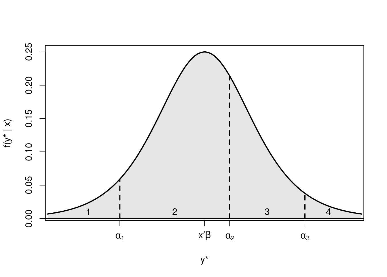
Figure 6.1: Distribution of the latent variable y* divided into four categories
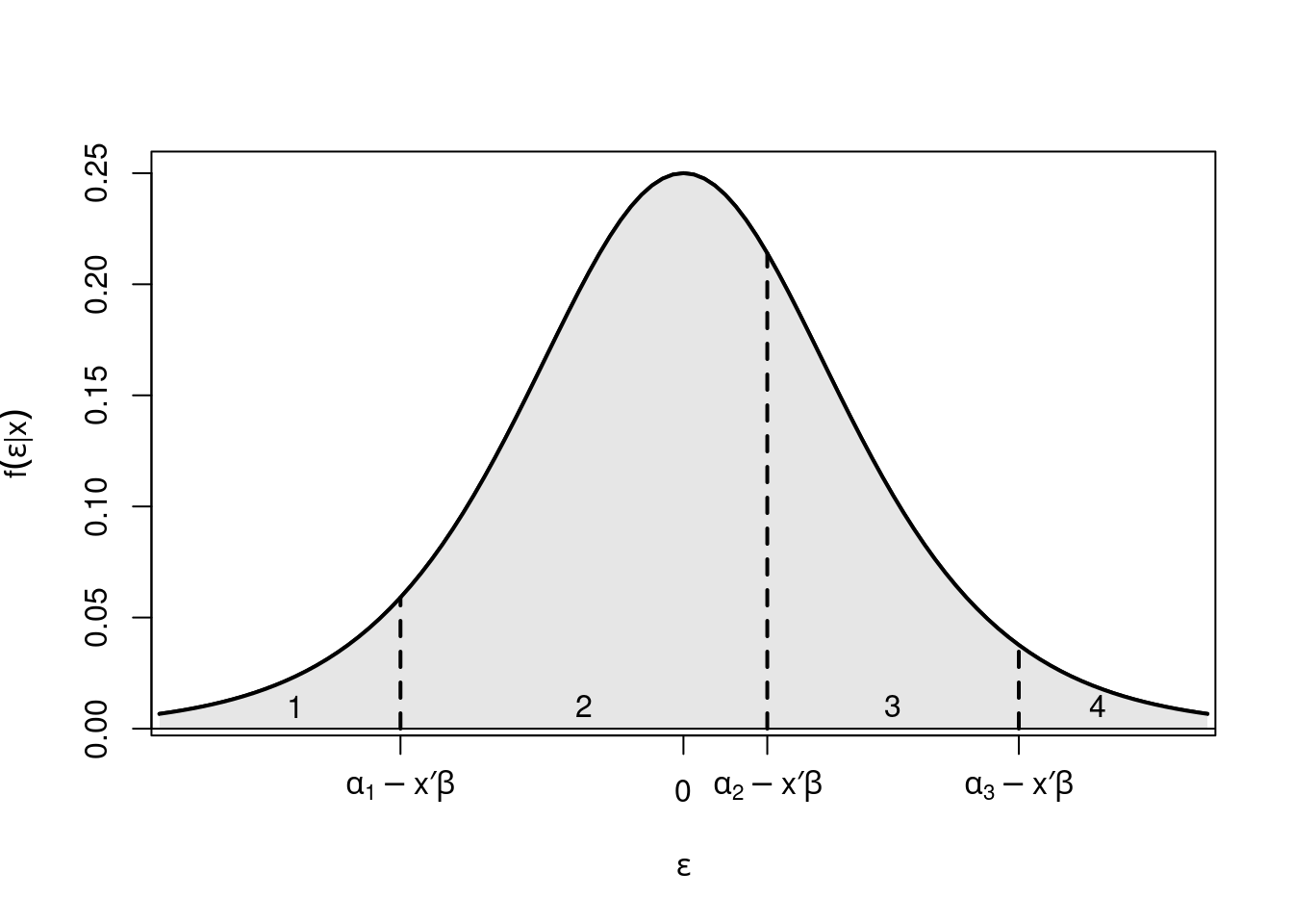
Figure 6.2: Distribution of the error term divided into four categories
Remember that we used a similar motivation in Chapter 4, where there might be an underlying continuous latent variable (e.g., willingness to buy a product), with a certain expectation plus an error term. The question is then whether the individual crosses a certain threshold, i.e., if he buys the product. In Chapter 4, we have also discussed that it is not possible to estimate this threshold and the intercept in the regression model. Thus, in the binary regression model we estimate the intercept and assume that the threshold to jump over is zero. In ordered models, the opposite is done: the intercept is not estimated, and therefore the threshold variables \(\alpha_j\) that need to be crossed to end up in the next category can be modeled explicitly. Note that in this case, \(x_i\) must not contain a constant, as the intercept is not identified.
We are only able to determine the relative, and not the absolute scale of the curve and the thresholds, which means the curve can be shifted left or right, depending the set of regressors, with the thresholds remaining at their original value. This results in persons with different sets of regressors having different probabilities of ending up in a given category. Note that even though the effect of a regressor on the latent scale is monotonic (positive or negative coefficient), its effect on the corresponding probabilities for the categories might not be monotonic. See on Figure 5.2: Shifting the curve to the right first increases the probability of category 3, but shifting it further to the right will eventually decrease it. Note, furthermore, that coefficients \(\beta\) do not depend on category \(j\), thus covariates have the same effect in all categories (single index).
Estimation: (Log-)Likelihood is as in the multinomial model, only with different parametrization of \(\pi_{ij}\).
\[\begin{eqnarray*} L(\alpha_1, \dots, \alpha_{m-1}, \beta; y, x) & = & \prod_{i = 1}^n f(y_i ~|~ x_i; \alpha_1, \dots, \alpha_{m-1}, \beta) \\ & = & \prod_{i = 1}^n \prod_{j = 1}^m \pi_{ij}^{d_{ij}} \\ \ell(\alpha_1, \dots, \alpha_{m-1}, \beta) & = & \sum_{i = 1}^n \sum_{j = 1}^m d_{ij} \cdot \log(\pi_{ij}) \qquad (\le 0). \end{eqnarray*}\]
6.2.1 Interpretation of parameters
Interpretation of parameters of an ordered response model on the underlying latent scale is straightforward and works similarly to a simple linear regression model: coefficients can be interpreted directly as the change in the response variable if a particular regressor changes by one unit. For example, with an underlying latent scale of risk aversion, we could say that risk aversion increases by \(\beta_1\) units if the regressor variable \(X_1\) (e.g., age) increases by one unit. The problem is that these units of risk aversion have no particular meaning, since they are for a latent variable that is never observed directly. What is usually of most interest in ordered response models is how the probabilities for individual categories change, but this is not so straightforward. We can calculate marginal probability effects for different categories:
\[\begin{equation*} \mathit{MPE}_{ijl} ~=~ \frac{\partial \pi_{ij}}{\partial x_{il}} ~=~ \{ h(\alpha_{j-1} - x_i^\top \beta) ~-~ h(\alpha_j - x_i^\top \beta) \} \cdot \beta_l, \end{equation*}\]
where the sign of the effect is only clear a priori for \(j = 1\) and \(j = m\), i.e., for the first and the last category. For categories in between: \(j = 2, \dots, m-1\) the sign depends on the thresholds.
Thus, ceterus paribus comparisons are only possible in ordered models:
- On the underlying latent scale
- For the cumulative probabilities (e.g., category 1. & 2. vs. category 3. & 4.)
- For the most extreme categories
Whereas for other individual categories, the sign of the change in probabilities is not determined by the sign of the regression coefficient.
Interpretation: Same ideas as in multinomial model.
- Assess influence in terms of probabilities. Either by calculating probabilities (i.e., effects) or investigating their partial changes (i.e., marginal effects).
- Compensating variation.
- For ordinal logit model: Odds or odds ratios.
Compensating variation: The linear predictor (and thus all probabilities) are unchanged if partial changes in regressors \(l\) and \(s\) cancel out, i.e.,
\[\begin{equation*} 0 ~=~ \beta_l \cdot \Delta x_{il} ~+~ \beta_s \cdot \Delta x_{is} \qquad \mbox{or} \qquad \frac{\Delta x_{il}}{\Delta x_{is}} ~=~ -\frac{\beta_s}{\beta_l}. \end{equation*}\]
Thus, for a single unit change in \(x_{is}\) a change of \(-\beta_s/\beta_l\) is required in \(x_{il}\) to keep resulting probabilities unchanged.
Odds: In the ordered logit model, the (log-)odds are expressed for cumulative probabilities, not individual ones.
\[\begin{eqnarray*} \log\left( \frac{\text{P}(y_i \le j ~|~ x_i)}{1 - \text{P}(y_i \le j ~|~ x_i)} \right) & = & \alpha_j ~-~ x_i^\top \beta, \\ \mathit{odds}(y_i \le j ~|~ x_i) & = & \exp(\alpha_j ~-~ x_i^\top \beta) ~=~ \exp(\alpha_j) \cdot \exp(-x_i^\top \beta). \end{eqnarray*}\]
Odds ratios: Odds ratios for different categories and different regressors, respectively:
\[\begin{eqnarray*} \frac{\mathit{odds}(y_i \le l ~|~ x_i)}{\mathit{odds}(y_i \le s ~|~ x_i)} & = & \exp(\alpha_l - \alpha_s), \\ \frac{\mathit{odds}(y_a \le j ~|~ x_a)}{\mathit{odds}(y_b \le j ~|~ x_b)} & = & \exp(-(x_a - x_b)^\top \beta), \end{eqnarray*}\]
hence the name proportional odds model. Log-odds just differ by a constant.
Interpretation of coefficients in terms of odds ratios: The odds for reaching \(j\) as the highest category change by a factor of \(\exp(\beta_l)\) for a single-unit change in the \(l\)-th regressor.
As we have seen in previous chapters, the logistic model is simpler to interpret with the help of odds and odds ratios. Furthermore, on the underlying latent scale, the ordered model is simpler to interpret than the unordered (multinomial) model, since coefficient \(\beta_l\) signals whether \(y_i^*\) increases/decreases in \(l\)-th regressor. However, influence of regressors on the individual probabilities for different categories \(\text{P}(y_i = j ~|~ x_i)\) is still not straightforward.
Note that the number of parameters in an ordered model, \(k + m - 1\), is lower than that in multinomial models, \((m - 1) \cdot (k + 1)\), as in the latter, a different set of regressors pertains to each category. Hence, try to exploit ordering information to build simpler models, if such information is available.
6.2.2 Example: Bank wages
As explained in the introduction, we are going to revisit the BankWages data, where categories of job can be regarded as being ordered: "custodial" \(<\) "admin" \(<\) "manage". Recall that only the subset of male employees was used in the previous chapter.
For an exploratory analysis, create a contingency table or corresponding mosaic displays.
##                    edcat  8 12 14-15 16-18 19-21
## minority job
## no       custodial        6  8     0     0     0
##          admin            6 30    66     7     1
##          manage           0  0     4    38    28
## yes      custodial        7  5     1     0     0
##          admin            4 18    18     7     0
##          manage           0  1     0     2     1
Visualize data using the joint distribution of all variables:
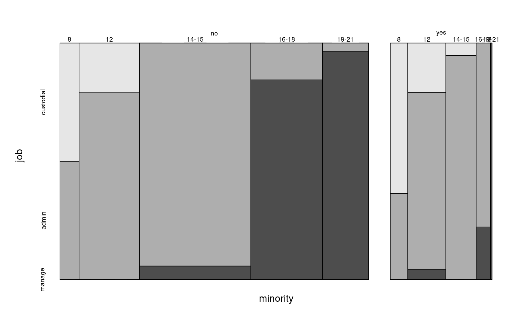
Figure 6.3: Mosaic plot of the Bank wages data
Alternatively, plot the conditional distribution given minority.
mosaicplot(bw_tab[1,,], off = 0, col = rev(gray.colors(3)),
  main = "minority = no")
mosaicplot(bw_tab[2,,], off = 0, col = rev(gray.colors(3)),
  main = "minority = yes")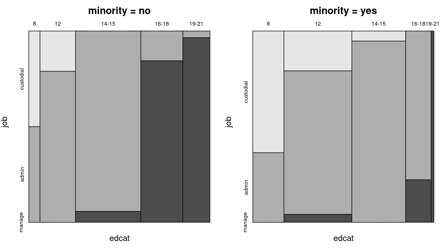
Figure 6.4: Job vs. education category for non-minority and minority employees
To set up the model, function polr() in package MASS provides ordinal models with logit (default) or probit link, among others. The name of the function derives from the default proportional odds logistic regression. Alternatively, function clm() in package ordinal provides the same models as well as some more flexibility, e.g., further link functions and structured thresholds. Furthermore, clmm() allows inclusion of random effects.
Model job category explained by education and minority variables:
library("MASS")
bw_olm <- polr(job ~ education + minority, data = bwmale,
  Hess = TRUE)
summary(bw_olm)
## Call:
## polr(formula = job ~ education + minority, data = bwmale, Hess = TRUE)
##
## Coefficients:
## Value Std. Error t value
## education 0.87 0.0931 9.35
## minorityyes -1.06 0.4120 -2.56
##
## Intercepts:
## Value Std. Error t value
## custodial|admin 7.951 1.077 7.383
## admin|manage 14.172 1.474 9.612
##
## Residual Deviance: 260.64
## AIC: 268.64The output contains no intercept, only the coefficients of education and minority, and the thresholds (or category-specific intercepts) between the three categories: one for custodial|admin and one for admin|management, which are necessarily ordered. Marginal effects and effect plots will be examined later in detail, but we can already see that on the latent scale of “qualification” underlying job category, education has a positive effect on qualification, while minority has a slightly negative effect.
Coefficient tests and likelihood ratio test:
##
## z test of coefficients:
##
##                 Estimate Std. Error z value Pr(>|z|)
## education         0.8700     0.0931    9.35  < 2e-16
## minorityyes      -1.0564     0.4120   -2.56     0.01
## custodial|admin   7.9514     1.0769    7.38  1.5e-13
## admin|manage 14.1721 1.4744 9.61 < 2e-16## Likelihood ratio test
##
## Model 1: job ~ education + minority
## Model 2: job ~ 1
## #Df LogLik Df Chisq Pr(>Chisq)
## 1 4 -130
## 2 2 -231 -2 202 <2e-16Ordered probit model can be fitted via
Or, in this case, simply with the update() function
Here, logit and probit models again give very similar results.
| Probit model | Logit model | |
|---|---|---|
| custodial|admin | 4.443 | 7.951 |
| (0.557) | (1.077) | |
| admin|manage | 7.844 | 14.172 |
| (0.744) | (1.474) | |
| education | 0.479 | 0.870 |
| (0.047) | (0.093) | |
| minorityyes | -0.509 | -1.056 |
| (0.214) | (0.412) | |
| Num.Obs. | 258 | 258 |
| AIC | 270.4 | 268.6 |
| BIC | 284.6 | 282.9 |
| RMSE | 1.97 | 1.97 |
## Likelihood ratio test
##
## Model 1: job ~ education + minority
## Model 2: job ~ 1
##   #Df LogLik Df Chisq Pr(>Chisq)
## 1   4   -131
## 2   2   -231 -2   200     <2e-16
To assess goodness of fit of the model, as before, confusion matrices can be computed, e.g., by employing majority voting.
##            pred
## true        custodial admin manage
##   custodial        13    14      0
##   admin            10   144      3
## manage 0 31 43## custodial admin manage
## 0.01726 0.88105 0.10169## [1] admin
## Levels: custodial admin manage6.2.3 Parallel regression assumption
A crucial assumption underlying standard ordered response models is the parallel regression assumption, which means regression coefficients \(\beta\) are the same across all categories \(j = 1, \dots, m\) (unlike we have seen in multinomial models). This, in turn, implies parallel regression lines for a given value \(\pi\) of the probabilities \(\pi_{ij}\). We have already discussed the intuition behind this: If the distribution on the latent scale is shifted across different thresholds, the way it shifts through any threshold is always the same, hence the probabilities going up and down for a certain category follow exactly the same pattern, which depends only on the link function. The slope at a given value \(0.5 = H(\alpha_j - x_i^\top \beta)\) with respect to linear predictor \(x_i^\top\) is
\[\begin{equation*} \frac{\partial \text{P}(y_i \le j ~|~ x_i)}{\partial x_i^\top \beta} ~=~ - h(\alpha_j - x_i^\top \beta) ~=~ -h(0). \end{equation*}\]
where \(h\) is the density function (normal or logistic). To sum up, since the regression coefficients are the same across all categories, the regression lines for success probabilities of different classes are parallel, which means the slopes of the probability curves are the same at a given value.
For a visualized example, we take a logistic model \(\text{P}(y_i \le j ~|~ x_i) = \Lambda(\alpha_j - x_i^\top \beta)\) with \(m = 4\), univariate \(x_i\), \(\alpha_1 = -2.7\), \(\alpha_2 = 0.8\), \(\alpha_3 = 3.2\), \(\beta = 1\). \(\pi\) for \(x_i = (\alpha_j - \Lambda^{-1}(\pi))/\beta\) with slope \(-\beta \cdot \lambda(\Lambda^{-1}(\pi))\).
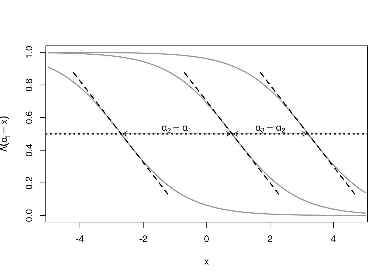
Figure 6.5: Logistic model - Parallel regression assumption
Above we can see three cumulative plots, where the first curve is the probability of \(y_i \leq 1\), e.g., the probability of ending up in a custodial job in the bank wages data, which decreases as the regressor \(x\) increases. The second line, \(\text{P}(y_i \leq 2)\)), is the probability of reaching at most the second category (or lower) e.g., reaching at most the admin category in the bank wages data, which also goes down as the regressor \(x\) increases, and so on for higher categories. Looking at the curves crossing 50% probability (where it is equally likely to fall below or above a certain category), we can see that the slopes are the same for all curves, and only depend on the density function corresponding to the link function being used. The differences between thresholds \(\alpha_2-\alpha_1, \alpha_3-\alpha_2\) determine how far the curves are shifted apart.
There are two ways of assessing the parallel regression assumption: (1) Compare the proportional odds logistic regression model (POLR) with an (unordered) multinomial logit model, or (2) Estimate \(m-1\) binary logit/probit models and compare them with the ordered model. Note however, that both of these assessments are informal (although formal tests could be developed based on the second idea). To formally compare multinomial and ordered models, the standard likelihood ratio- or Wald tests cannot be employed since the two models are not nested. There are two ways to deal with this: using a generalized ordered response model (more flexible), or relying on information criteria - AIC, BIC - rather than formal tests.
6.2.4 Example: Bank wages
Comparing the multinomial and the ordered logit- and probit models for the bank wages data in terms of AIC:
library("nnet")
bw_mnl <- multinom(job ~ education + minority, data = bwmale,
  trace = FALSE)
AIC(bw_mnl, bw_olm, bw_opm)
## df AIC
## bw_mnl 6 249.5
## bw_olm 4 268.6
## bw_opm 4 270.4## df AIC
## bw_mnl 6 270.8
## bw_olm 4 282.9
## bw_opm 4 284.6The AIC of the multinomial (unordered) model is the lowest. The ordered logit- and probit models perform very similarly in terms if AIC, and somewhat worse than the multinomial. In addition, even by increasing penalty to \(log(n)\) to compute BIC, the multinomial model performs better. Note that in this case it would be possible to use the BIC() function instead of specifying the penalty formula in the AIC() function, but not all model classes support the former.
Corresponding effects plots:
library("effects")
eff_mnl <- allEffects(bw_mnl, xlevels = list(education = 50))
eff_olm <- allEffects(bw_olm, xlevels = list(education = 50))
plot(eff_olm, multiline = TRUE)Bank wages effects: Ordered model
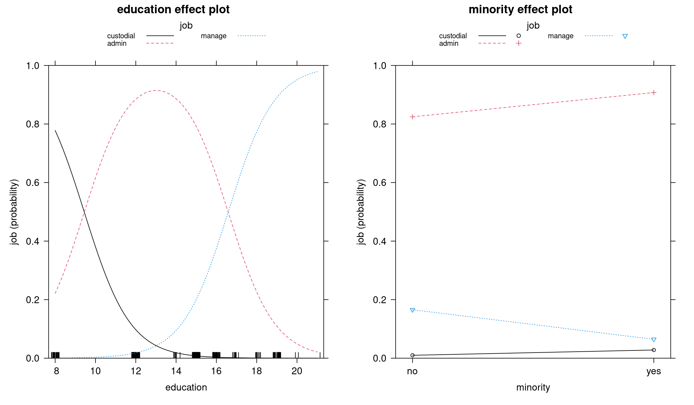
Figure 6.6: Education and minority effect plots - Ordered model
Bank wages effects: Multinomial model
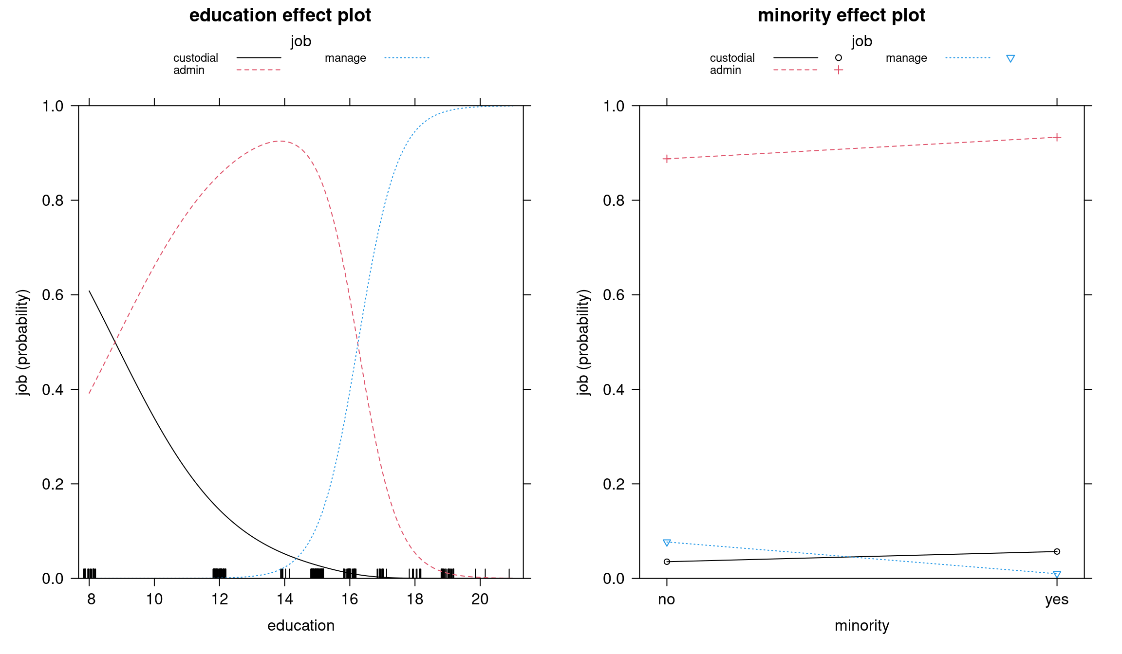
Figure 6.7: Education and minority effect plots - Multinomial model
In both models, the transition between admin and management is sharp: if you cross a certain level of education, the probability of working in management suddenly goes up. There is a relatively clear education effect going on between these two categories, whereas between custodial and admin we cannot say the same: custodial workers are not promoted to admin category after more education, it is simply a different trajectory. However, in the proportional odds model, the two curves are parallel, and there is no possibility to have different effects at different thresholds, which is why in this case the multinomial model fits better.
We can see the same in stacked effect pots:
Bank wages: Stacked effect plots (Ordered model)
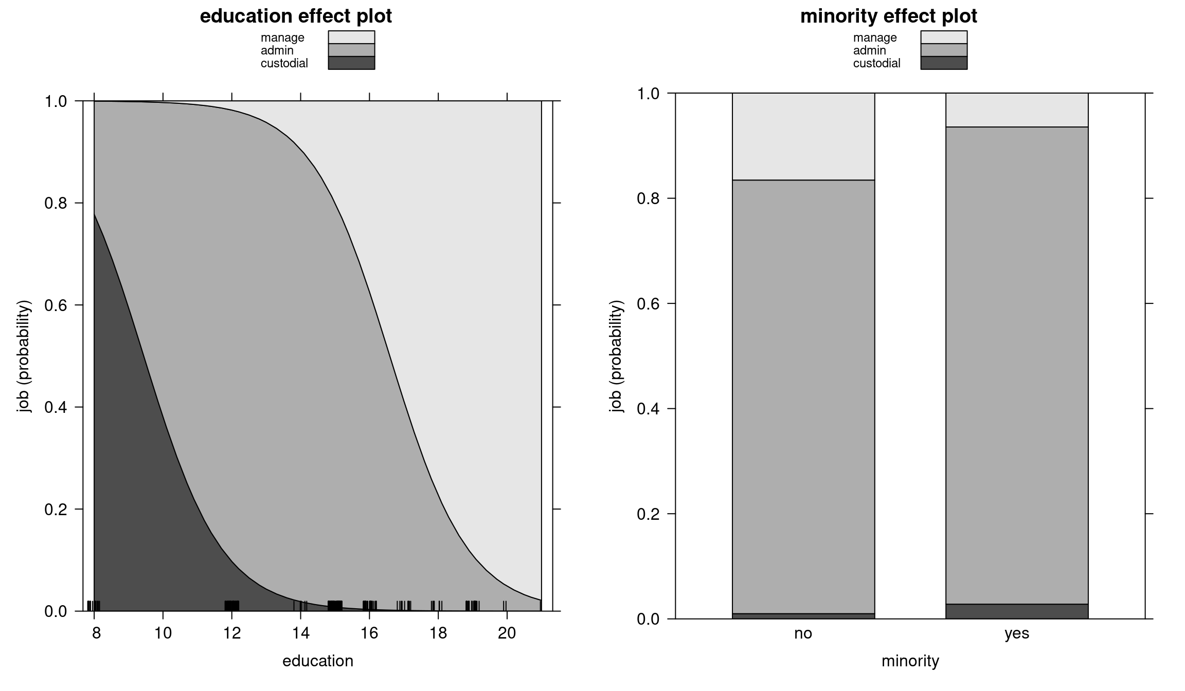
Figure 6.8: Education and minority stacked effect plots - Ordered model
Bank wages: Stacked effect plots (Multinomial model)
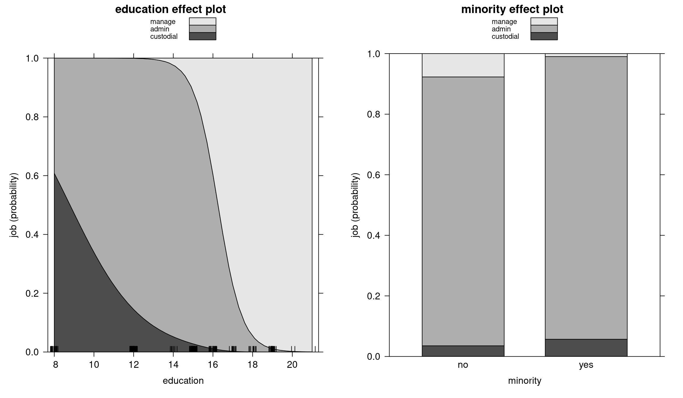
Figure 6.9: Education and minority stacked effect plots - Multinomial model
Contingency tables to assess accuracy: multinomial and ordered model predictions
##            pred
## true        custodial admin manage
##   custodial        13    14      0
##   admin            10   138      9
## manage 0 7 67## pred
## true custodial admin manage
## custodial 13 14 0
## admin 10 144 3
## manage 0 31 43Estimate \(m-1=2\) binary logit models and compare them with the ordered model:
We now estimate two binary logit models - one for every threshold, where we get different intercepts for each category, but we also get different slope parameters for each of the thresholds. We set up one binary model for the response custodial vs. “not custodial”, and one for the response manage vs. “not manage”.
bw_logit1 <- glm(I(job != "custodial") ~ education + minority,
  family = binomial, data = bwmale)
bw_logit2 <- glm(I(job == "manage") ~ education + minority,
  family = binomial, data = bwmale)
modelsummary(list("Custodial/Not custodial"=bw_logit1,
                  "Manage/Not manage"=bw_logit2),
fmt=3, estimate="{estimate}{stars}")| Custodial/Not custodial | Manage/Not manage | |
|---|---|---|
| (Intercept) | -5.062*** | -26.215*** |
| (1.148) | (4.312) | |
| education | 0.586*** | 1.645*** |
| (0.095) | (0.277) | |
| minorityyes | -0.481 | -2.120** |
| (0.509) | (0.794) | |
| Num.Obs. | 258 | 258 |
| AIC | ||
| BIC | ||
| Log.Lik. | ||
| F | 20.052 | 18.155 |
| RMSE | 0.26 | 0.26 |
To conclude, the parallel regression assumption appears to be violated in this case, meaning POLR and ordered probit models are not suitable for this data set. As explained before, this result is plausible due to the presumably different latent processes responsible for "custodial" vs. "admin" and "admin" vs. "manage", respectively.
6.3 Extensions
In current practice, ordered logit and probit models are predominantly used, as they are relatively easy to interpret. However, there are two main problems with using these models:
- Single index and parallel regression assumption.
- Threshold parameters \(\alpha_j\) are constant across all individuals \(i\), i.e., do not depend on covariates.
Hence, generalizations that overcome these problems should be considered. However, these are not easily available in software packages.
6.3.1 Generalized Threshold Models
In generalized threshold models, the threshold parameters are linear functions of the covariates.
\[\begin{equation*} \alpha_{ij} ~=~ \tilde \alpha_j ~+~ x_i^\top \gamma_j \end{equation*}\]
Probability model:
\[\begin{eqnarray*} \pi_{ij} & = & H(\tilde \alpha_j ~+ x_i^\top \gamma_j ~-~ x_i^\top \beta) ~-~ H(\tilde \alpha_{j-1} ~+ x_i^\top \gamma_{j-1} ~-~ x_i^\top \beta) \\ & = & H(\tilde \alpha_j ~-~ x_i^\top \beta_j) ~-~ H(\tilde \alpha_{j-1} ~-~ x_i^\top \beta_{j-1}) \end{eqnarray*}\]
where \(\beta_j = \beta - \gamma_j\) as \(\beta\) and \(\gamma_j\) cannot be identified separately.
Note that standard ordered models are nested within this generalized model class (unlike MNL). Hence, testing of \(\beta_1 = \dots = \beta_{m-1}\) is possible using standard methods.
6.3.2 Sequential models
Some ordinal variables capture categories that can only be reached successively, e.g., university degrees (Bachelor is a necessary prerequisite to Master’s degree). Then, it is possible to model transition probabilities, i.e., the probability of remaining in a certain category \(y_i = j\) given that at least this category was reached \(y_i \le j\).
Probability model:
\[\begin{equation*} \text{P}(y_i = j ~|~ y_i \ge j,~ x_i) ~=~ H(\alpha_j ~-~ x_i^\top \beta). \end{equation*}\]
Again, category-specific parameters \(\beta_j\) could be employed to generalize the model.