Chapter 3 Maximum Likelihood Estimation
3.1 Introduction
In our setup for this chapter, population distribution is known up to the unknown parameter(s). The task is then to estimate parameters, and thus full population distribution from an empirical sample. We are going to denote observations \(y_i\) (\(i = 1, \dots, n\)), from probability density function \(f(y_i; \theta)\) with parameter \(\theta \in \Theta\). Under independence, the joint probability function of the observed sample can be written as the product over individual probabilities:
\[\begin{equation*} f(y_1, \dots, y_n; \theta) ~=~ \prod_{i = 1}^n f(y_i; \theta) \end{equation*}\]
Note that we present unconditional models, as they are easier to introduce. Extension to conditional models \(f(y_i ~|~ x_i; \theta)\) does not change fundamental principles, but their implementation is more complex.
3.2 Likelihood Function
The joint probability density for observing \(y_1, \dots, y_n\) given \(\theta\) is called the joint distribution. Alternatively, as a function of the unknown parameter \(\theta\) given a random sample \(y_1, \dots, y_n\), this is called the likelihood function of \(\theta\).
\[\begin{equation*} L(\theta) ~=~ L(\theta; y_1, \dots, y_n) ~=~ f(y_1, \dots, y_n; \theta) %% ~=~ \prod_{i = 1}^n L(\theta; y_i) %% ~=~ \prod_{i = 1}^n f(y_i; \theta) \end{equation*}\]
The idea of maximum likelihood estimation is to find the set of parameters \(\hat \theta\) so that the likelihood of having obtained the actual sample \(y_1, \dots, y_n\) is maximized. The maximum likelihood estimator \(\hat \theta_{ML}\) is then defined as the value of \(\theta\) that maximizes the likelihood function.
\[\begin{equation*} \hat \theta ~=~ \underset{\theta \in \Theta}{argmax} L(\theta) \end{equation*}\]
It is important to distinguish between an estimator and the estimate. The ML estimator (MLE) \(\hat \theta\) is a random variable, while the ML estimate is the value taken for a specific data set. Also note that more generally, any function proportional to \(L(\theta)\) – i.e., any \(c \cdot L(\theta)\) – can serve as likelihood function. Fisher (1922) defined likelihood in his description of the method as:
“The likelihood that any parameter (or set of parameters) should have any assigned value (or set of values) is proportional to the probability that if this were so, the totality of observations should be that observed.”
— Fisher, 1922
In practice, we most often use the log-likelihood, rather than the likelihood itself:
\[\begin{equation*} \ell(\theta) ~=~ \log L(\theta) %% ~=~ \sum_{i = 1}^n \log f(y_i; \theta) \end{equation*}\]
The log-likelihood is a monotonically increasing function of the likelihood, therefore any value of \(\hat \theta\) that maximizes likelihood, also maximizes the log likelihood. As mentioned in Chapter 2, the log-likelihood is analytically more convenient, for example when taking derivatives, and numerically more robust, which becomes important when dealing with very small or very large joint densities. Under independence, products are turned into computationally simpler sums by using log-likelihood.
\[\begin{eqnarray*} L(\theta; y) ~=~ L(\theta; y_1, \dots, y_n) & = & \prod_{i = 1}^n L(\theta; y_i) ~=~ \prod_{i = 1}^n f(y_i; \theta) \\ \ell(\theta; y) ~=~ \ell(\theta; y_1, \dots, y_n) & = & \sum_{i = 1}^n \ell(\theta; y_i) ~=~ \sum_{i = 1}^n \log f(y_i; \theta). \end{eqnarray*}\]
3.2.1 Score function and Hessian matrix
The Score function is the first derivative (or gradient) of log-likelihood, sometimes also simply called score. We denote it as \(s(\theta; y) ~=~ \frac{\partial \ell(\theta; y)}{\partial \theta}\). The Hessian matrix is the second derivative of log-likelihood, \(\frac{\partial^2 \ell(\theta; y)}{\partial \theta \partial \theta^\top}\), denoted as \(H(\theta; y)\). Under independence, the log-likelihood function is additive, thus the Score function and the Hessian matrix are also additive.
\[\begin{eqnarray*} s(\theta; y_1, \dots, y_n) & = & \sum_{i = 1}^n s(\theta; y_i) \\ H(\theta; y_1, \dots, y_n) & = & \sum_{i = 1}^n H(\theta; y_i) \end{eqnarray*}\]
3.2.2 Maximization
Typically we assume that the parameter space in which \(\theta\) lies is \(\Theta = \mathbb{R}^p\) with \(p \ge 1\). Thus, \(\Theta\) is unbounded and MLE might not exist even if \(\ell(\theta)\) is continuous. However, if there is an interior solution to the problem, we solve the first-order conditions for a maximum, i.e., we set the score function, which is the first derivative of the log-likelihood, to 0.
\[\begin{equation*} s(\hat \theta; y) ~=~ 0. \end{equation*}\]
For a necessary and sufficient condition we require \(H(\hat \theta)\) (the Hessian matrix) to be negative definite. This is always fulfilled in “well-behaved cases”, i.e., when \(\ell(\theta)\) is log-concave. This means that the solution to the first-order condition gives a unique solution to the maximization problem.
3.2.3 Example: Bernoulli experiment
Assume that a random sample of size n has been drawn from a Bernoulli distribution. Then,
\[\begin{eqnarray*} L(\pi; y) & = & \prod_{i = 1}^n \pi^{y_i} (1 - \pi)^{1 - y_i} \\ \ell(\pi; y) & = & \sum_{i = 1}^n (1 - y_i) \log(1 - \pi) ~+~ y_i \log \pi \\ s(\pi; y) & = & \sum_{i = 1}^n \frac{y_i - \pi}{\pi (1 - \pi)} \\ H(\pi; y) & = & \sum_{i = 1}^n - \frac{y_i}{\pi^2} - \frac{1 - y_i}{(1 - \pi)^2} \end{eqnarray*}\]
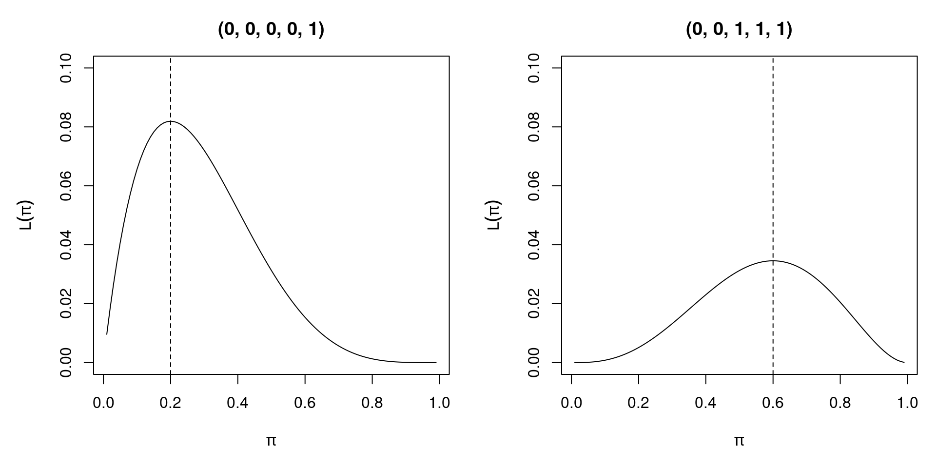
Figure 3.1: Likelihood Function of Two Different Bernoulli Samples
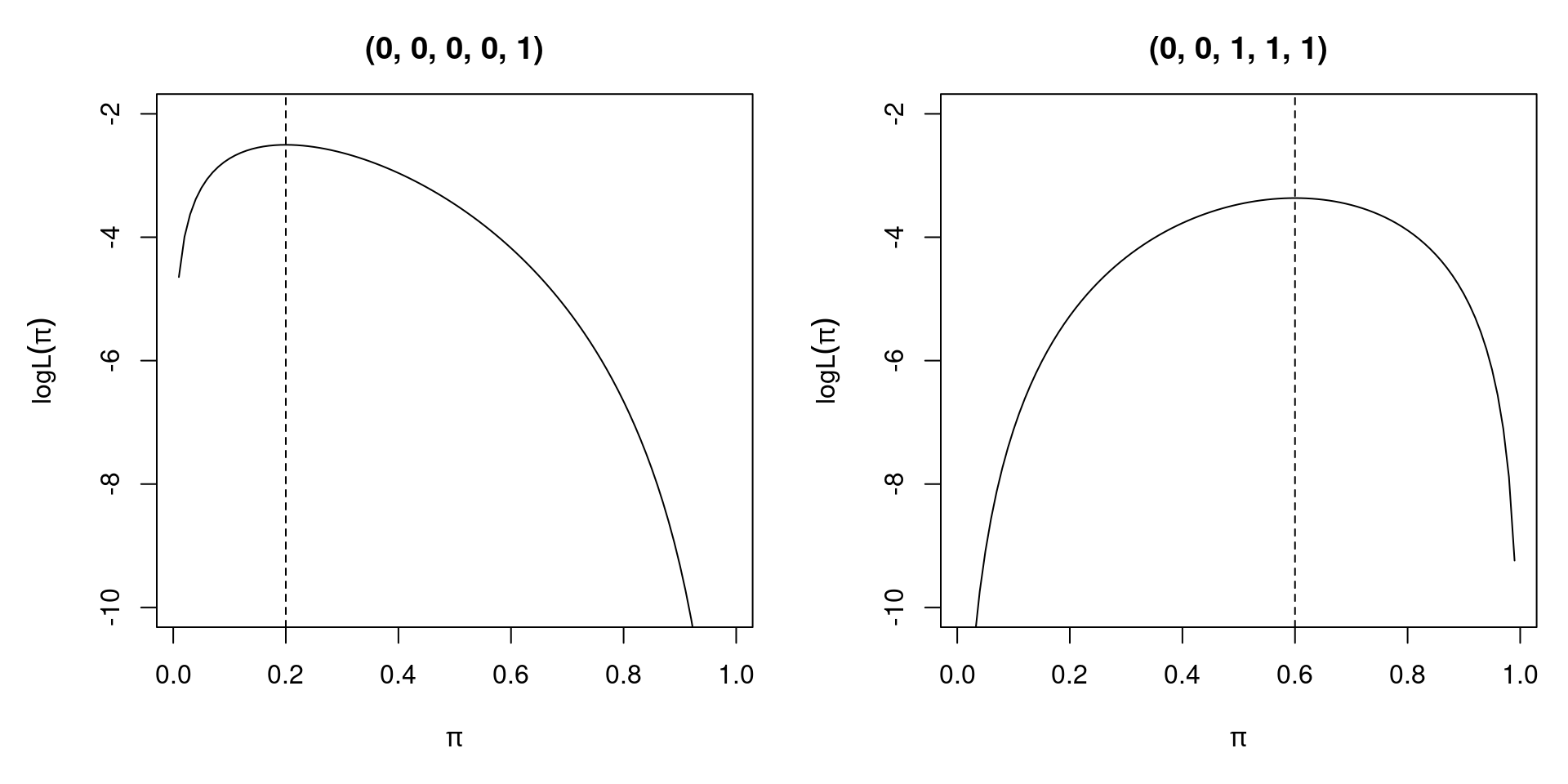
Figure 3.2: Log - Likelihood of Two Different Bernoulli Samples
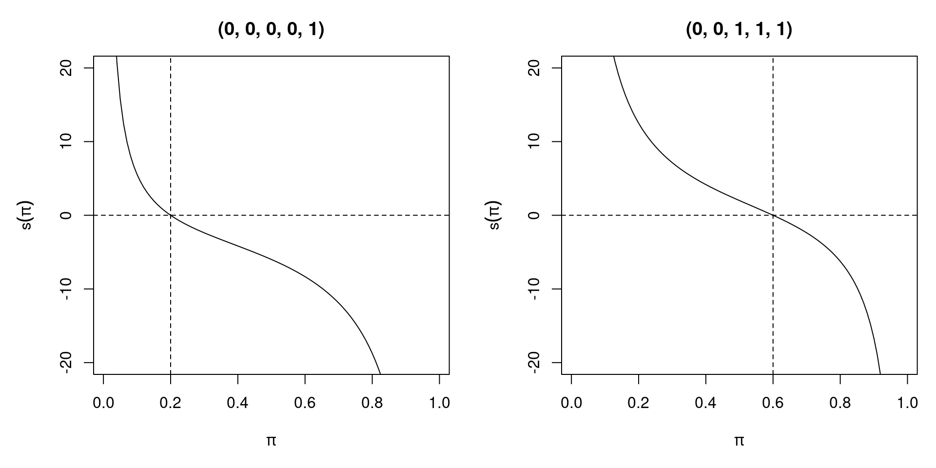
Figure 3.3: Score Function of Two Different Bernoulli Samples
Solving the first order condition, we see that the MLE is given by \(\hat \pi ~=~ \frac{1}{n} \sum_{i = 1}^n y_i\), the sample mean. The Hessian matrix \(H(\hat \pi)\) is negative as long as there is variation in \(y_i\). Then, an interior solution with a well-defined score and Hessian exists. Without variation (i.e., all \(y_i = 0\) or all \(y_i = 1\)), \(\hat \pi\) is on the boundary of the parameter space and the model fits perfectly. In the Bernoulli case with a conditional logit model, perfect fit of the model breaks down the maximum likelihood method because 0 or 1 cannot be attained by
\[\begin{equation*} \pi_i ~=~ \text{logit}^{-1} (x_i^\top \beta) ~=~ \frac{\exp(x_i^\top \beta)}{1 + \exp(x_i^\top \beta)}. \end{equation*}\]
3.3 Properties of the Maximum Likelihood Estimator
Let’s now turn our attention to studying the conditions under which it is sensible to use the maximum likelihood method. The questions we can ask are whether the MLE exists, if it is unique, unbiased and consistent, if it uses the information from the data efficiently, and what its distribution is. Unfortunately, there is no unified ML theory for all statistical models/distributions, but under certain regularity conditions and correct specification of the model (misspecification discussed later), MLE has several desirable properties:
- Consistency: As the sample size \(n\) increases, MLE tends to true parameter value \(\theta_0\).
- Asymptotic normality: In large samples, MLE has an approximate normal distribution around \(\theta_0\).
- Efficiency: MLE has smaller asymptotic variance than other consistent uniformly asymptotically normal estimators.
With large enough data sets, using asymptotic approximation is usually not an issue, however, in small samples MLE is typically biased.
3.3.1 ML regularity condition
A crucial assumption for ML estimation is the ML regularity condition:
\[\begin{equation*} 0 ~=~ \frac{\partial}{\partial \theta} \int f(y_i; \theta) ~ dy_i ~=~ \int \frac{\partial}{\partial \theta} f(y_i; \theta) ~ dy_i, \end{equation*}\] i.e., the order of integration and differentiation can be interchanged. This is fulfilled if the domain of integration is independent of \(\theta\) e.g., for exponential family distributions. However, exceptions exist, e.g., uniform distribution on \([0, \theta]\). Regularity condition implies that the expected score evaluated at the true parameter \(\theta_0\) is equal to zero.
\[\begin{equation*} E \{ s(\theta_0; y_i) \} ~=~ 0, \end{equation*}\]
3.3.2 Consistency
The consistency of ML estimation follows from the ML regularity condition. Under random sampling, the score is a sum of independent components. Thus, by the law of large numbers, the score function converges to the expected score. MLE is then picked such that sample score is zero. Since in the expected score, zero is only attained at true value \(\theta_0\), it follows that \(\hat \theta \overset{\text{p}}{\longrightarrow} \theta_0\).
3.3.3 Example: Bernoulli experiment
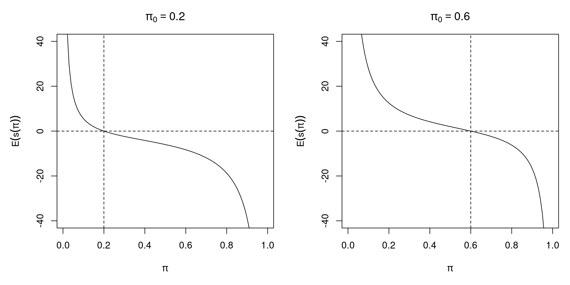
Figure 3.4: Expected Score of Two Different Bernoulli Samples
The expected score function is \(\text{E} \{ s(\pi; y_i) \} ~=~ \frac{n (\pi_0 - \pi)}{\pi (1 - \pi)}\)
3.3.4 Fisher information
To investigate the variance of MLE, we define the Fisher information as the variance of the score:
\[\begin{equation*} I(\theta) ~=~ Cov \{ s(\theta) \} \end{equation*}\]
The Fisher information is important for assessing identification of a model. Furthermore, it is the inverse of the variance of the maximum likelihood estimator. It also links maximum likelihood estimation to the Cramer-Rao lower bound, which is the lower bound on the variance of unbiased estimators, and is given by the inverse of the Fisher information. The maximum likelihood estimator reaches the Cramer-Rao lower bound, therefore it is asymptotically efficient. A further result related to the Fisher information is the so-called information matrix equality, which states that under maximum likelihood regularity condition, \(I(\theta_0)\) can be computed in several ways, either via first derivatives, as the variance of the score function, or via second derivatives, as the negative expected Hessian (if it exists), both evaluated at the true parameter \(\theta_0\):
\[\begin{eqnarray*} I(\theta_0) & = & \text{E} \{ s(\theta_0) s(\theta_0)^\top \}, \\ & = & \text{E} \{ - H(\theta_0) \} \end{eqnarray*}\]
Matrix \(J(\theta) = -H(\theta)\) is called observed information.
3.3.5 Asymptotic distribution
Under correct specification of the model, the ML regularity condition, and additional technical assumptions, \(\hat \theta\) converges in distribution to a normal distribution. More precisely,
\[\begin{equation*} \sqrt{n} ~ (\hat \theta - \theta_0) \overset{\text{d}}{\longrightarrow} \mathcal{N}(0, A_0^{-1}), \end{equation*}\]
where the asymptotic covariance matrix \(A_0\) depends on the Fisher information
\[\begin{equation*} A_0 ~=~ \lim_{n \rightarrow \infty} \left( - \frac{1}{n} E \left[ \left. \sum_{i = 1}^n \frac{\partial^2 \ell(\theta; y_i)}{\partial \theta \partial \theta^\top} \right] \right|_{\theta = \theta_0} \right) ~=~ \lim_{n \rightarrow \infty} \frac{1}{n} I(\theta_0), \end{equation*}\]
i.e., \(A_0\) is the “asymptotic average information” in an observation. In practice, for “large” \(n\), we use
\[\begin{equation*} \hat \theta ~\approx~ \mathcal{N}\left( \theta_0, \frac{1}{n} A_0^{-1} \right) ~=~ \mathcal{N}(\theta_0, I^{-1}(\theta_0)), \end{equation*}\]
which is a compact way of stating all three essential properties of the maximum likelihood estimator: consistency (due to the mean), efficiency (due to variance), and asymptotic normality (due to distribution). However, we still need an estimator for \(I(\theta_0)\).
As mentioned earlier, some technical assumptions are necessary for the application of the central limit theorem. Namely, the model needs to be identified, i.e., \(f(y; \theta_1) = f(y; \theta_2) \Leftrightarrow \theta_1 = \theta_2\), and the log likelihood needs to be three times differentiable. Furthermore, we assume existence of all matrices (e.g., Fisher information), and a “well-behaved” parameter-space \(\Theta\). In addition, we assume that the ML regularity condition (interchangeability of the order differentiation and integration) holds. In conditional models, further assumptions about the regressors are required.
3.3.6 Covariance matrix
The asymptotic covariance matrix of the MLE can be estimated in various ways. Due to information matrix equality, \(A_0 = B_0\), where
\[\begin{equation*} B_0 ~=~ \lim_{n \rightarrow \infty} \frac{1}{n} \text{E} \left[ \left. \sum_{i = 1}^n \frac{\partial \ell(\theta; y_i)}{\partial \theta} \frac{\partial \ell(\theta; y_i)}{\partial \theta^\top} \right] \right|_{\theta = \theta_0}. \end{equation*}\]
Estimation can be based on different empirical counterparts to \(A_0\) and/or \(B_0\), which are asymptotically equivalent.
The two different estimators based on the second order derivatives are:
Expected information:
\[\begin{equation*} \hat{A_0} ~=~ - \frac{1}{n} \left. E \left[ \sum_{i = 1}^n \frac{\partial^2 \ell(\theta; y_i)}{\partial \theta \partial \theta^\top} \right] \right|_{\theta = \hat \theta} ~=~ \frac{1}{n} I(\hat \theta). \end{equation*}\]
Observed information:
\[\begin{equation*} \hat{A_0} ~=~ - \frac{1}{n} \left. \sum_{i = 1}^n \frac{\partial^2 \ell(\theta; y_i)}{\partial \theta \partial \theta^\top} \right|_{\theta = \hat \theta} ~=~ \frac{1}{n} J(\hat \theta). \end{equation*}\]
Alternatively, we can use analogous estimators based on first order derivatives.:
\[\begin{equation*} \hat{B_0} ~=~ \frac{1}{n} \left. E \left[ \sum_{i = 1}^n \frac{\partial \ell(\theta; y_i)}{\partial \theta} \frac{\partial \ell(\theta; y_i)}{\partial \theta^\top} \right] \right|_{\theta = \hat \theta}. \end{equation*}\] or \[\begin{equation*} \hat{B_0} ~=~ \frac{1}{n} \left. \sum_{i = 1}^n \frac{\partial \ell(\theta; y_i)}{\partial \theta} \frac{\partial \ell(\theta; y_i)}{\partial \theta^\top} \right|_{\theta = \hat \theta}. \end{equation*}\]
Where the latter is also called “outer product of gradient” (OPG) or estimator of Berndt, Hall, Hall, and Hausman (BHHH). In practice, there is no widely accepted preference for observed vs. expected information. OPG is simpler to compute but is typically not used if observed/expected information is available. Modern software typically reports observed information as it is generally a product of numerical optimization.
3.3.7 Example: Fitting distributions
As an example in R, we are going to fit a parameter of a distribution via maximum likelihood. We use data on strike duration (in days) using exponential distribution, which is the basic distribution for durations.
\[\begin{equation*} f(y; \lambda) ~=~ \lambda \exp(-\lambda y), \end{equation*}\]
where \(y > 0\) and \(\lambda > 0\) the scale parameter.
In R, dexp() with parameter rate. Fitting via fitdistr() in package MASS.
data("StrikeDuration", package = "AER")
library("MASS")
(fit <- fitdistr(StrikeDuration$duration, densfun = "exponential"))
## rate
## 0.023432
## (0.002976)## 'log Lik.' -294.7 (df=1)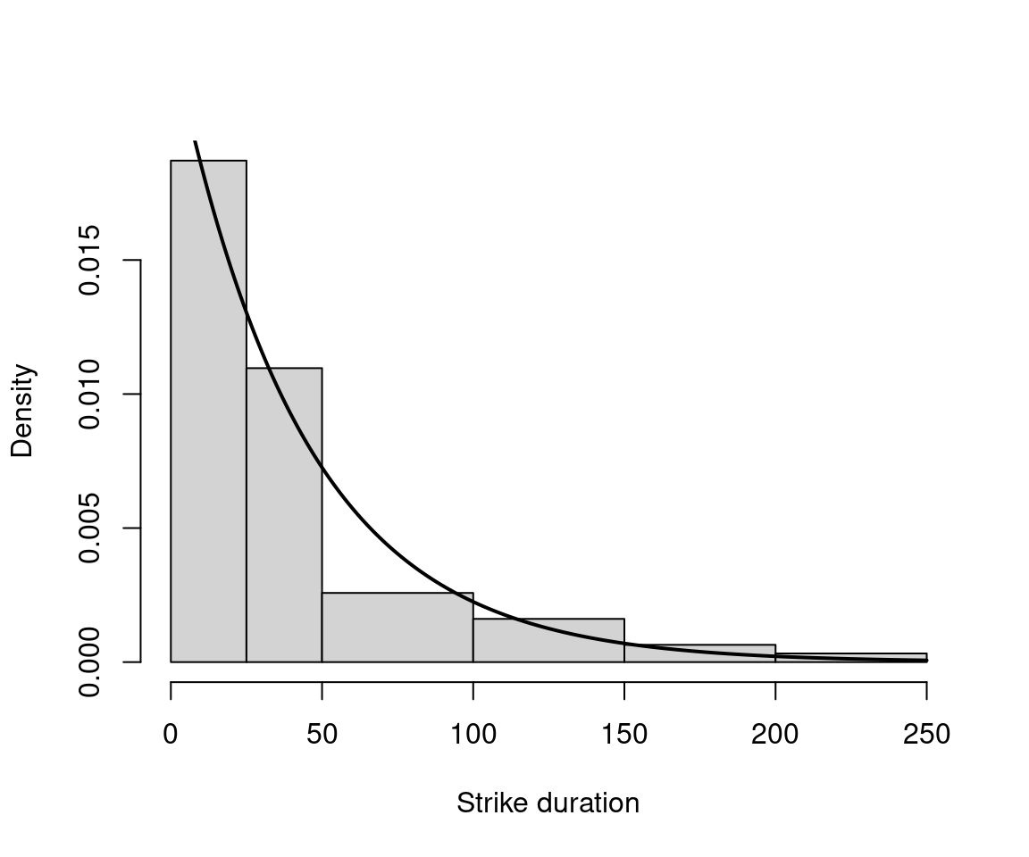
Figure 3.5: Distribution of Strike Duration
3.4 Normal Linear Model
The linear regression model \(y_i = x_i^\top \beta + \varepsilon_i\) with normally independently distributed (n.i.d.) errors can be written as
\[\begin{equation*} y_i ~|~ x_i ~\sim ~ \mathcal{N}(x_i^\top \beta, \sigma^2) \quad \mbox{independently}. \end{equation*}\]
This implies: \[\begin{eqnarray*} f(y_i ~| x_i; \beta, \sigma^2) & = & \frac{1}{\sqrt{2 \pi \sigma^2}} ~ \exp \left\{ -\frac{1}{2} ~ \frac{(y_i - x_i^\top \beta)^2}{\sigma^2} \right\}, \\ \ell(\beta, \sigma^2) & = & -\frac{n}{2} \log(2 \pi) ~-~ \frac{n}{2} \log(\sigma^2) ~-~ \frac{1}{2 \sigma^2} \sum_{i = 1}^n (y_i - x_i^\top \beta)^2. \end{eqnarray*}\]
The first order conditions are:
\[\begin{eqnarray*} \frac{\partial \ell}{\partial \beta} & = & \frac{1}{\sigma^2} \sum_{i = 1}^n x_i (y_i - x_i^\top \beta) ~=~ 0, \\ \frac{\partial \ell}{\partial \sigma^2} & = & - \frac{n}{2 \sigma^2} ~+~ \frac{1}{2 \sigma^4} \sum_{i = 1}^n (y_i - x_i^\top \beta)^2 ~=~ 0. \end{eqnarray*}\]
Thus, \(\hat \beta_\text{ML} = \hat \beta_\text{OLS}\) is
\[\begin{equation*} \hat \beta ~=~ \left( \sum_{i = 1}^n x_i x_i^\top \right)^{-1} \sum_{i = 1}^n x_i y_i. \end{equation*}\]
Furthermore, with \(\hat \varepsilon_i = y_i - x_i^\top \hat \beta\),
\[\begin{equation*} \hat{\sigma}^2 ~=~ \frac{1}{n} \sum_{i = 1}^n \hat \varepsilon_i^2. \end{equation*}\]
The Hessian matrix is \[\begin{equation*} H(\beta, \sigma^2) ~=~ \left( \begin{array}{cc} -\frac{1}{\sigma^2} \sum_{i = 1}^n x_i x_i^\top & -\frac{1}{\sigma^4} \sum_{i = 1}^n x_i (y_i - x_i^\top \beta) \\ -\frac{1}{\sigma^4} \sum_{i = 1}^n x_i (y_i - x_i^\top \beta) & \frac{n}{2 \sigma^4} - \frac{1}{\sigma^6} \sum_{i = 1}^n (y_i - x_i^\top \beta)^2 \end{array} \right). \end{equation*}\]
Thus, the information matrix is \[\begin{equation*} I(\beta, \sigma^2) ~=~ E \{ -H(\beta, \sigma^2) \} ~=~ \left( \begin{array}{cc} \frac{1}{\sigma^2} \sum_{i = 1}^n x_i x_i^\top & 0 \\ 0 & \frac{n}{2 \sigma^4} \end{array} \right). \end{equation*}\]
Therefore, the asymptotic covariance matrix of the MLE is \[\begin{equation*} I(\beta, \sigma^2)^{-1} ~=~ \left( \begin{array}{cc} \sigma^2 \left( \sum_{i = 1}^n x_i x_i^\top \right)^{-1} & 0 \\ 0 & \frac{2 \sigma^4}{n} \end{array} \right). \end{equation*}\]
Stronger assumptions (compared to Gauss-Markov, i.e., the additional assumption of normality) yield stronger results: with normally distributed error terms, \(\hat \beta\) is efficient among all consistent estimators. This distributional assumption is not critical for the quality of estimator, though: ML\(=\)OLS, i.e., moment restrictions are sufficient for obtaining good estimator. Thus, some misspecification is not critical. However, the normal linear model is atypical because a closed-form solution exists for the maximum likelihood estimator. For most microdata models, however, such a closed-form solution is not applicable, and thus numerical methods have to be employed.
3.5 Further Aspects of Maximum Likelihood Estimation
3.5.1 Invariance
To study invariance, we examine what the ML estimator of a (potentially nonlinear) function of \(h(\theta)\) is. The invariance property says that the ML estimator of \(h(\theta)\) is simply the function evaluated at MLE for \(\theta\):
\[\begin{equation*} \widehat{h(\theta)} ~=~ h(\hat \theta), \end{equation*}\]
For example, in the Bernoulli case, find MLE for \(Var(y_i) = \pi (1 - \pi) = h(\pi)\). As \(\hat \pi = \bar y\), use \(h(\hat \pi) = \bar y (1 - \bar y)\).
3.5.2 Delta method
To find the covariance matrix of \(h(\hat \theta)\), we use the Delta method (if \(h(\theta)\) is differentiable):
\[\begin{equation*} \sqrt{n} ~ (h(\hat \theta) - h(\theta_0)) \overset{\text{d}}{\longrightarrow} \mathcal{N} \left(0, \left. \frac{\partial h(\theta)}{\partial \theta} \right|_{\theta = \theta_0} A_0^{-1} \left. \frac{\partial h(\theta)}{\partial \theta} \right|_{\theta = \theta_0}^\top \right). \end{equation*}\]
In practice, for “large” \(n\), we use
\[\begin{equation*} h(\hat \theta) ~\approx~ \mathcal{N} \left( h(\theta_0), \left. \frac{\partial h(\theta)}{\partial \theta} \right|_{\theta = \hat \theta} J^{-1}(\hat \theta) \left. \frac{\partial h(\theta)}{\partial \theta} \right|_{\theta = \hat \theta}^\top \right). \end{equation*}\]
3.5.3 Numerical optimization
To obtain MLE in empirical samples, there are various strategies that are conceivable:
- Trial and error (formalized as grid search, typically very inefficient).
- Graphical methods (only useful for 1- or maybe 2-dimensional \(\theta\)).
- Analytical optimization (efficient, but typically not available in closed form).
- Numerical methods (based on numerical mathematics).
A common element of numerical optimization algorithms is that they are typically iterative and require specification of a starting value. A frequently used numerical optimization method is the Newton-Raphson method, which will be described in further detail here:
Let \(h: \mathbb{R} \rightarrow \mathbb{R}\) differentiable (sufficiently often). What we want is \(x\) with \(h(x) = 0\). We thus employ Taylor expansion for \(x_0\) close to \(x\),
\[\begin{equation*} 0 ~=~ h(x) ~\approx~ h(x_0) ~+~ h'(x_0) (x - x_0) \end{equation*}\]
Solving for \(x\) yields
\[\begin{equation*} x ~\approx~ x_0 ~-~ \frac{h(x_0)}{h'(x_0)}. \end{equation*}\]
We then improve some approximate solution \(x^{(k)}\) for \(k = 1, 2, 3, \dots\),
\[\begin{equation*} x^{(k + 1)} ~=~ x^{(k)} ~-~ \frac{h(x^{(k)})}{h'(x^{(k)})}. \end{equation*}\]
Based on starting value \(x^{(1)}\), we iterate until some stop criterion fulfilled, e.g., \(|h(x^{(k)})|\) small or \(|x^{(k + 1)} - x^{(k)}|\) small. To transfer this to the maximum likelihood problem, based on starting value \(\hat \theta^{(1)}\), we iterate for \(k = 1, 2, \dots\),
\[\begin{equation*} \hat \theta^{(k + 1)} ~=~ \hat \theta^{(k)} ~-~ H(\hat \theta^{(k)})^{-1} s(\hat \theta^{(k)}) \end{equation*}\]
until \(|s(\hat \theta^{(k)})|\) is small or \(|\hat \theta^{(k + 1)} - \hat \theta^{(k)}|\) is small.
In the Newton-Raphson algorithm, the actual Hessian of the sample is used, evaluated at the current parameter value. We can, however, employ other estimators of the information matrix. We can employ the observed information: \(J(\hat \theta^{(k)})^{-1}\), or the expected information \(I(\hat \theta^{(k)})^{-1}\) (associated algorithm is then known as Fisher scoring in statistics), or the outer product of gradients: \(B(\hat \theta^{(k)})^{-1}\), which is also known in econometrics as the BHHH method.
3.5.4 Identification
There are two potential problems that can cause standard maximum likelihood estimation to fail. The first one is no variation in the data (in either the dependent and/or the explanatory variables). An example for this would be the previously discussed (quasi-)complete separation in binary regressions yielding perfect predictions. The second possible problem is lack of identification. Lack of identification results in not being able to draw certain conclusions, even in infinite samples.
“Identification problems cannot be solved by gathering more of the same kind of data. These inferential difficulties can be alleviated only by invoking stronger assumptions or by initiating new sampling processes that yield different kinds of data.”
(Manski, 1995)
There are several types of identification failure that can occur, for example identification by exclusion restriction. If there are too many parameters, such as
\[\begin{equation*} E(y_i ~|~ \mathit{male}_i, \mathit{female}_i) ~=~ \beta_0 + \beta_1 \mathit{male}_i + \beta_2 \mathit{female}_i. \end{equation*}\]
Not all parameters are identified for such dummy variables because \(\mathit{male}_i = 1 - \mathit{female}_i\). The solution for the lack of identification here is to impose a restriction, e.g., to either omit the intercept (\(\beta_0 = 0\)), to impose treatment contrasts (\(\beta_1 = 0\) or \(\beta_2 = 0\)), or to use sum contrasts (\(\beta_1 + \beta_2 = 0\)). A second type of identification failure is identification by functional form. For the sampling of \(y_i\) given \(x_i = 1, 2\), one can identify \(E(y_i ~|~ x_i = 1)\) and \(E(y_i ~|~ x_i = 2)\). Then, without further assumptions \(E(y_i ~|~ x_i = 1.5)\) is not identified. The two possible solutions to overcome this problem are either to sample \(x_i = 1.5\) as well, or to assume a particular functional form, e.g., \(E(y_i ~|~ x_i) = \beta_0 + \beta_1 x_i\). The third type of identification problem is identification by probability models. Two parameters are observationally equivalent if \(f(y; \theta_1) = f(y; \theta_2)\) for all \(y\). A parameter point \(\theta_0\) is identifiable if there is no other \(\theta \in \Theta\) which is observationally equivalent.
3.5.5 Quasi-maximum likelihood
The most important problem with maximum likelihood estimation is that all desirable properties of the MLE come at the price of strong assumptions, namely the specification of the true probability model. What are the properties of the MLE when the wrong model is employed? In the linear regression model, various levels of misspecification (distribution, second or first moments) lead to loss of different properties. However, many problems can be remedied, and we know that the estimator remains useful under milder assumptions as well. Here, we will employ model \(\mathcal{F} = \{f_\theta, \theta \in \Theta\}\) but let’s say the true density is \(g \not\in \mathcal{F}\). Then the maximum likelihood estimator is called pseudo-MLE or quasi-MLE (QMLE). One can then ask if the QMLE is still consistent, what its distribution is, and what an appropriate covariance matrix estimator would be. MLE solves the first order conditions:
\[\begin{equation*} s(\theta) ~=~ \frac{\partial \ell(\theta)}{\partial \theta} ~=~ \sum_{i = 1}^n \frac{\partial \ell_i(\theta)}{\partial \theta} ~=~ 0 \end{equation*}\]
Intuitively, MLE \(\hat \theta\) is consistent for \(\theta_0 \in \Theta\) if
\[\begin{equation*} \frac{1}{n} \sum_{i = 1}^n \frac{\partial \ell_i(\hat \theta)}{\partial \theta} ~\overset{\text{p}}{\longrightarrow}~ 0 ~=~ \text{E}_0 \left( \frac{\partial \ell(\theta_0)}{\partial \theta} \right) ~=~ \int \frac{\partial \log f(y_i; \theta_0)}{\partial \theta} ~ f(y_i; \theta_0) ~ dy_i. \end{equation*}\]
However, if \(g \not\in \mathcal{F}\) is the true density, then
\[\begin{equation*} \frac{1}{n} \sum_{i = 1}^n \frac{\partial \ell_i(\hat \theta)}{\partial \theta} ~\overset{\text{p}}{\longrightarrow}~ 0 ~=~ \text{E}_g \left( \frac{\partial \ell(\theta_*)}{\partial \theta} \right) ~=~ \int \frac{\partial \log f(y_i; \theta_*)}{\partial \theta} ~ g(y_i) ~ dy_i \end{equation*}\]
for some \(\theta_* \in \Theta\). This \(\theta_*\) is called pseudo-true value.
What is the relationship between \(\theta_*\) and \(g\), then? Under regularity conditions,
\[\begin{eqnarray*} 0 & = & \text{E}_g \left( \frac{\partial \log f(y; \theta)}{\partial \theta} \right) ~=~ \int \frac{\partial \log f(y; \theta)}{\partial \theta} ~ g(y) ~ dy \\ & = & \frac{\partial}{\partial \theta} \int \log f(y; \theta) ~ g(y) ~ dy \\ & = & \dots ~=~ \frac{\partial}{\partial \theta} \int \log \left( \frac{g(y)}{f(y; \theta)} \right) ~ g(y) ~ dy \\ & = & \frac{\partial}{\partial \theta} K(g, f_\theta). \end{eqnarray*}\]
where \(K(g, f) = \int \log(g/f) g(y) dy\) is the Kullback-Leibler distance from \(g\) to \(f\), also known as Kullback-Leibler information criterion (KLIC). Therefore, QMLE solves first order conditions for the optimization problem
\[\begin{equation*} \underset{\theta \in \Theta}{argmin} K(g, f_\theta). \end{equation*}\]
There is still consistency, but for something other than originally expected. QMLE is consistent for \(\theta_*\) which corresponds to the distribution \(f_{\theta_*} \in \mathcal{F}\) with the smallest Kullback-Leibler distance from \(g\), but \(g \neq f_{\theta_*}\). Under regularity conditions, the following (asymptotic normality) holds
\[\begin{equation*} \sqrt{n} ~ (\hat \theta - \theta_*) ~\overset{\text{d}}{\longrightarrow}~ \mathcal{N}(0, A_*^{-1} B_* A_*^{-1}), \end{equation*}\]
where
\[\begin{eqnarray*} A_* & = & - \lim_{n \rightarrow \infty} \frac{1}{n} E \left. \left[ \sum_{i = 1}^n \frac{\partial^2 \ell_i(\theta)}{\partial \theta \partial \theta^\top} \right] \right|_{\theta = \theta_*} \\ B_* & = & \underset{n \rightarrow \infty}{plim} \frac{1}{n} \sum_{i = 1}^n \left. \frac{\partial \ell_i(\theta)}{\partial \theta} \frac{\partial \ell_i(\theta)}{\partial \theta^\top} \right|_{\theta = \theta_*} \end{eqnarray*}\]
Thus, the covariance matrix is of sandwich form, and the information matrix equality does not hold anymore. A special case is exponential families, where the ML estimator is typically still consistent for parameters pertaining to the conditional expectation function, as long as it is correctly specified, but the covariance matrix is more complicated. However, valid sandwich covariances can often be obtained. For independent observations, the simplest sandwich standard errors are also called Eicker-Huber-White sandwich standard errors, sometimes also referred to as subsets of the names, or simply as robust standard errors. Important examples of this in econometrics include OLS regression and Poisson regression. In linear regression, for example, we can use heteroscedasticity consistent (HC) covariances.
\[\begin{eqnarray*} n \hat{A_*} & = & - \frac{1}{\sigma^2} \sum_{i = 1}^n x_i x_i^\top, \\ n \hat{B_*} & = & \frac{1}{\sigma^4} \sum_{i = 1}^n \hat \varepsilon_i^2 x_i x_i^\top. \end{eqnarray*}\]
Therefore,
\[\begin{equation*} A_*^{-1} B_* A_*^{-1} ~=~ \left( \frac{1}{n} \sum_{i = 1}^n x_i x_i^\top \right)^{-1} \left( \frac{1}{n} \sum_{i = 1}^n \hat \varepsilon_i^2 x_i x_i^\top \right) \left( \frac{1}{n} \sum_{i = 1}^n x_i x_i^\top \right)^{-1}. \end{equation*}\]
3.6 Testing
Inference refers to the process of drawing conclusions about population parameters, based on estimates from an empirical sample. Typically, we are interested in parameters that drive the conditional mean, and scale or dispersion parameters (e.g., \(\sigma^2\) in linear regression, \(\phi\) in GLM) are often treated as nuisance parameters. To test a hypothesis, let \(\theta \in \Theta = \Theta_0 \cup \Theta_1\), and test
\[\begin{equation*} H_0: ~ \theta \in \Theta_0 \quad \mbox{vs.} \quad H_1: ~ \theta \in \Theta_1. \end{equation*}\]
Or, written as restriction of parameters space,
\[\begin{equation*} H_0: ~ R(\theta) = 0 \quad \mbox{vs.} \quad H_1: ~ R(\theta) \neq 0, \end{equation*}\]
for \(R: \mathbb{R}^p \rightarrow \mathbb{R}^{q}\) with \(q < p\).
A special case is the linear hypothesis \(H_0: R \theta = r\) with \(R \in \mathbb{R}^{q \times p}\). We denote the unrestricted MLE (under \(H_1\)) by \(\hat \theta\), and the restricted MLE by \(\tilde \theta\). Analogously, the estimate of the asymptotic covariance matrix for \(\hat \theta\) is \(\hat V\), and \(\tilde V\) is the estimate for \(\tilde \theta\), for example \(\hat{A_0}\), \(\hat{B_0}\), or some kind of sandwich estimator. Finally, \(\hat R = \left. \frac{\partial R(\theta)}{\partial \theta} \right|_{\theta = \hat \theta}\). As an example, let’s examine a log-linear wage function:
\[\begin{equation*} \log(\mathtt{wage}) ~=~ \beta_0 ~+~ \beta_1 \mathtt{education} ~+~ \beta_2 \mathtt{experience} ~+~ \beta_3 \mathtt{experience}^2 ~+~ \varepsilon \end{equation*}\]
Typical hypotheses would be \(\beta_1 = 0\) (‘education’ not in model, given ‘experience’) or \(\beta_1 = 0.06\) (return to schooling is 6 % per year).
To conduct a likelihood ratio test, we estimate the model both under \(H_0\) and \(H_1\), then check
\[\begin{equation*} \ell(\hat \theta) ~\approx~ \ell(\tilde \theta). \end{equation*}\]
For a Wald test, we estimate the model only under \(H_1\), then check
\[\begin{equation*} R(\hat \theta) ~\approx~ 0. \end{equation*}\]
And finally, to conduct a score test, we estimate the model only under \(H_0\) and check
\[\begin{equation*} s(\tilde \theta) ~\approx~ 0. \end{equation*}\]
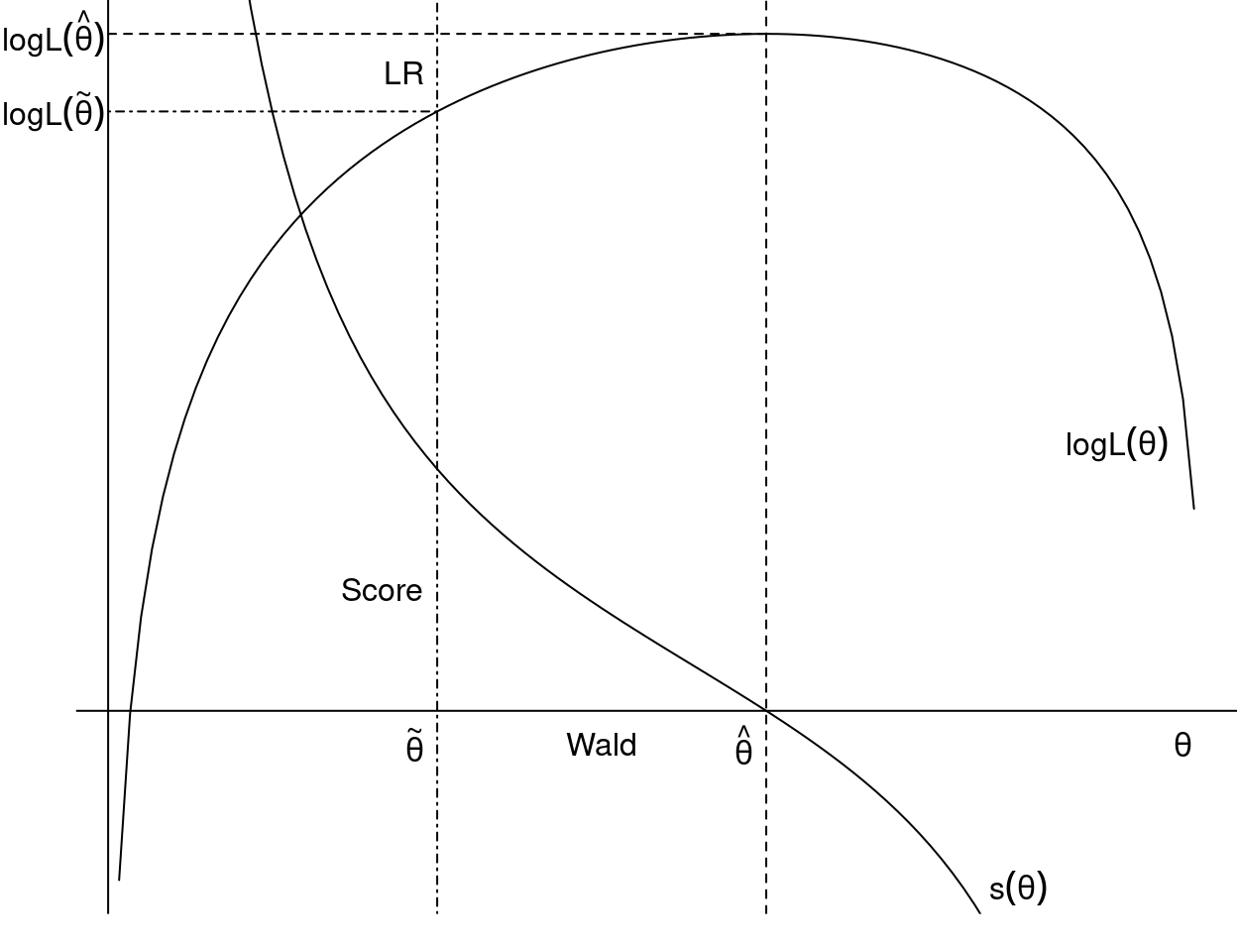
Figure 3.6: Score Test, Wald Test and Likelihood Ratio Test
The Likelihood ratio test, or LR test for short, assesses the goodness of fit of two statistical models based on the ratio of their likelihoods, and it examines whether a smaller or simpler model is sufficient, compared to a more complex model. \(H_0\) is to be rejected if
\[\begin{equation*} \mathit{LR} ~=~ \frac{\max_{\theta \in \Theta} L(\theta)}{\max_{\theta \in \Theta_0} L(\theta)} \end{equation*}\]
is too large. Under \(H_0\) and technical assumptions
\[\begin{equation*} 2 \log \mathit{LR} ~=~ -2 ~ \{ \ell(\tilde \theta) ~-~ \ell(\hat \theta) \} ~\overset{\text{d}}{\longrightarrow}~ \chi_{p - q}^2 \end{equation*}\]
i.e., the LR test statistics is Chi-square distributed with \(p-q\) degrees of freedom, from which critical values and \(p\) values can be computed. The likelihood ratio test may be elaborate because both models need to be estimated, however, it is typically easy to carry out for nested models in R. Note that two models are nested if one model contains all predictors of the other model, plus at least one additional one.
The Wald test (named after Abraham Wald) assesses constraints on statistical parameters based on the weighted distance between the unrestricted estimate and its value under \(H_0\). We employ
\[\begin{equation*} R(\hat \theta)^\top (\hat R \hat V \hat R^\top)^{-1} R(\hat \theta) ~\overset{\text{d}}{\longrightarrow}~ \chi_{p - q}^2 \end{equation*}\]
In the special case of a linear restriction \(R \theta = r\):
\[\begin{equation*} (R \hat \theta - r)^\top (R \hat V R^\top)^{-1} (R \hat \theta - r) ~\overset{\text{d}}{\longrightarrow}~ \chi_{p - q}^2 \end{equation*}\]
The Wald test is convenient if the null hypothesis is a nonlinear restriction, because the alternative hypothesis is often easier to compute than \(H_0\).
The Score test, or Lagrange-Multiplier (LM) test, assesses constraints on statistical parameters based on the score function evaluated at the parameter value under \(H_0\). Employ
\[\begin{equation*} s(\tilde \theta)^\top \tilde V s(\tilde \theta) ~\overset{\text{d}}{\longrightarrow}~ \chi_{p - q}^2 \end{equation*}\]
The score test is convenient to use if the alternative is complicated but null hypothesis is easy to estimate.
All three tests assess the same question, that is, does leaving out some explanatory variables reduce the fit of the model significantly? The advantage of the Wald- and the score test is that they require only one model to be estimated. All three tests asymptotically equivalent, meaning as \(n \rightarrow \infty\), the values of the Wald- and score test statistics will converge to the LR test statistic.
3.6.1 Model selection
To assess the problem of model selection, i.e., which model fits best, it is important to note that the objective function \(L(\hat \theta)\) or \(\ell(\hat \theta)\) is always improved when parameters are added (or restrictions removed). Therefore, the idea is to penalize increasing complexity (additional variables) via
\[\begin{equation*} \mathit{IC}(\theta) ~=~ -2 ~ \ell(\theta) ~+~ \text{penalty}, \end{equation*}\]
where the penalty increases with the number of parameters \(p\). Then, choose the “best” model by minimizing \(\mathit{IC}(\theta)\).
Important and most used special cases of penalizing are:
- Akaike information criterion (AIC), where penalty \(= 2 \cdot p\).
- Bayesian information criterion of Schwarz (BIC, SIC, or SBC), with a stricter penalty of \(= \log(n) \cdot p\).
3.6.2 Implementation in R
Many model-fitting functions in R employ maximum likelihood for estimation. Interfaces vary across packages but many of them supply methods to the following basic generic functions:
| Function | Description |
|---|---|
coef() |
extract estimated parameters \(\hat \theta\) |
vcov() |
extract estimated variance-covariance matrix, typically \(\frac{1}{n} J(\hat \theta)\) |
logLik() |
extract log-likelihood \(\ell(\hat \theta)\) (with attribute for \(p\)) |
AIC() |
compute information criteria including AIC, BIC/SBC; by default relies on logLik() method; allows specification of k for penalty \(= k \cdot p\) |
This set of extractor functions is extended in package sandwich:
| Function | Description |
|---|---|
estfun() |
extract matrix with \((s_1(\hat \theta), \dots, s_n(\hat \theta))\) |
bread() |
extract estimated \(\hat{A_0}\), typically \(J(\hat \theta)\) |
sandwich() |
compute sandwich estimator, by default based on bread() and cross-product of estfun() |
General inference tools are available in package lmtest and car. These are based on the availability of methods for logLik(), coef(), vcov(), among others.
| Function | Description |
|---|---|
lrtest() |
compute LR test for nested models |
waldtest() |
compute Wald test for nested models |
coeftest() |
compute partial Wald tests for each element of \(\theta\) |
linearHypothesis() |
compute Wald tests for linear hypotheses |
deltaMethod() |
compute Wald tests for nonlinear hypotheses by means of Delta method |
Finally, the packages modelsummary, effects, and marginaleffects provide general infrastructure for summarizing and visualizing models, including models fitted by maximum likelihood. The modelsummary package creates tables of estimated parameters, standard errors, and optionally test statistics, and exports them to a wide range of formats, including Markdown and LaTeX. The effects and marginaleffects packages create visualizations and tables that facilitate interpretation of parameters in regression models, which is particularly helpful in nonlinear models.
3.6.3 Example: Fitting distributions
As an example, we fit a Weibull distribution for strike duration (in days),
\[\begin{equation*} f(y; \alpha, \lambda) ~=~ \lambda ~ \alpha ~ y^{\alpha - 1} ~ \exp(-\lambda y^\alpha), \end{equation*}\] where \(y > 0\), \(\lambda > 0\), and \(\alpha > 0\) shape parameter. Hazard is increasing for \(\alpha > 1\), decreasing for \(\alpha < 1\) and constant for \(\alpha = 1\). Note that a Weibull distribution with a parameter \(\alpha = 1\) is an exponential distribution.
In R, dweibull() with parameter shape (\(= \alpha\)) and scale (\(= 1/\lambda\)). Fitting via fitdistr().
##     shape      scale
##    0.92468   41.10765
## ( 0.09156) ( 5.96082)## 'log Lik.' -294.4 (df=2)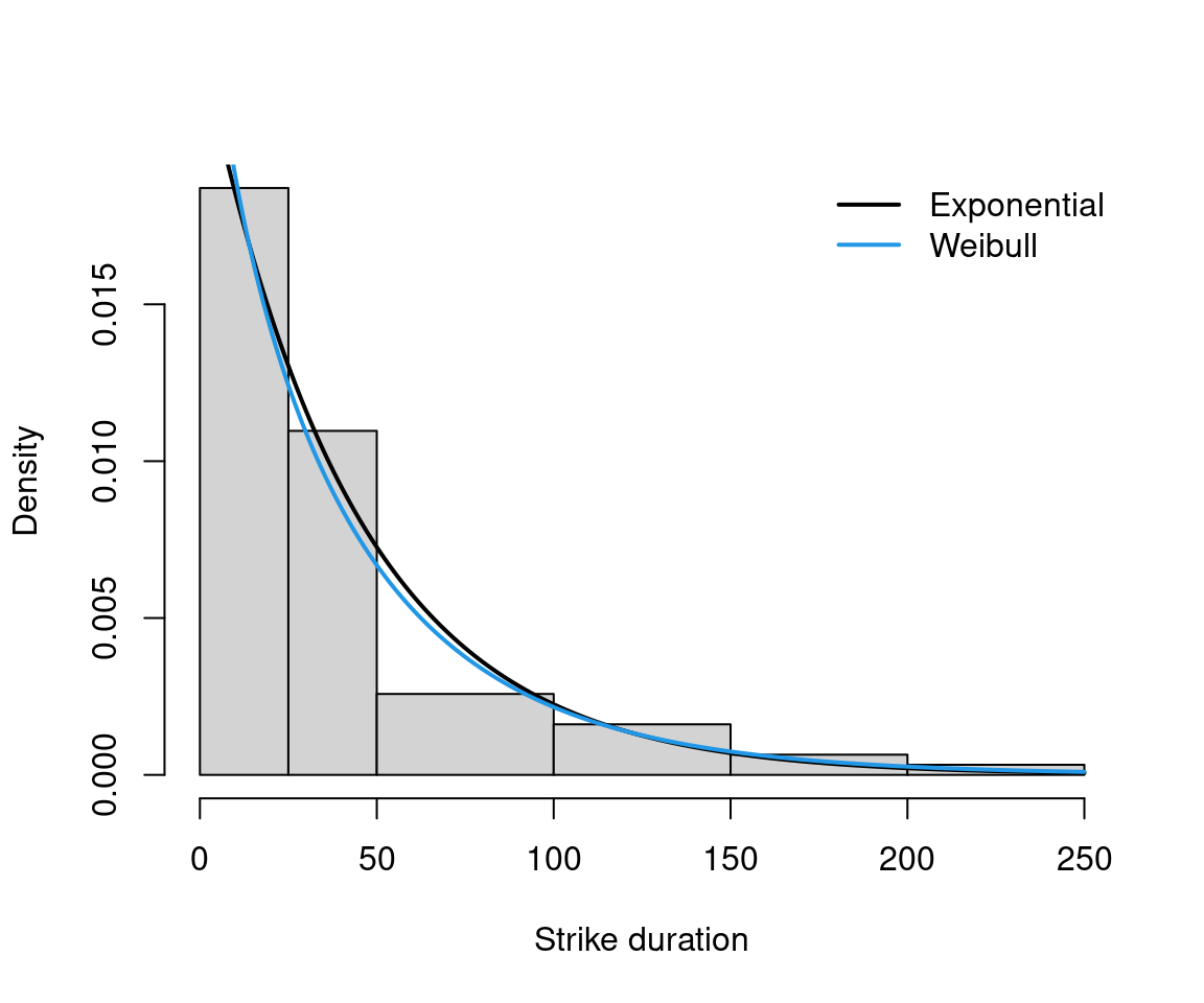
Figure 3.7: Fitting Weibull and Exponential Distribution for Strike Duration
##
## Linear hypothesis test:
## shape = 1
##
## Model 1: restricted model
## Model 2: fit2
##
##   Df Chisq Pr(>Chisq)
## 1
## 2 1 0.68 0.41## Likelihood ratio test
##
## Model 1: rate = 0.02
## Model 2: shape = 0.92, scale = 41.11
## #Df LogLik Df Chisq Pr(>Chisq)
## 1 1 -295
## 2 2 -294 1 0.65 0.42## df AIC
## fit 1 591.5
## fit2 2 592.8## df AIC
## fit 1 593.6
## fit2 2 597.1## df BIC
## fit 1 593.6
## fit2 2 597.1The estimate and standard error for \(\lambda = 1/\mathtt{scale}\) can also be obtained easily by applying the delta method with \(h(\theta) = \frac{1}{\theta}\), \(h'(\theta) = -\frac{1}{\theta^2}\). Then:
\(\widehat{Var(h(\hat \theta))} = \left(-\frac{1}{\hat \theta^2} \right) \widehat{Var(\hat \theta)} \left(-\frac{1}{\hat \theta^2} \right) = \frac{\widehat{Var(\hat \theta)}}{\hat \theta^4}\).
##    scale    scale
## 0.024326 0.003527
Or via deltaMethod() for both fit and fit2:
##        Estimate    SE 2.5 % 97.5 %
## 1/rate 42.68 5.42 32.05 53.3## Estimate SE 2.5 % 97.5 %
## 1/scale 0.02433 0.00353 0.01741 0.033.7 Pros and Cons of Maximum Likelihood
There are numerous advantages of using maximum likelihood estimation. Its use is convenient, as only the likelihood is required, and, if necessary, first and second derivatives can be obtained numerically. Furthermore, the underlying large-sample theory is well-established, with asymptotic normality, consistency and efficiency. Inference is simple using maximum likelihood, and the invariance property provides a further advantage. However, maximum likelihood estimation has its drawbacks as well. We need strong assumptions as the data-generating process needs to be known up to parameters, which is difficult in practice, as the underlying economic theory often provides neither the functional form, nor the distribution. Moreover, maximum likelihood estimation is not robust against misspecification or outliers.