Chapter 9 Duration Models

9.1 Introduction

Examples: Typical economic examples for duration responses.

Macroeconomics.
\(t_i\): Duration of strike \(i\).
Potential covariates: Macroeconomic indicators, …
Labor economics
\(t_i\): Duration of unemployment of person \(i\).
Potential covariates: Education, age, gender, …
Marketing.
\(t_i\): Duration between two purchases of person \(i\).
Potential covariates: Price, price of alternative products, …
Demography/population economics.
\(t_i\): Age of woman \(i\) at birth of first child.
Potential covariates: Education, income, …

Remarks:

Duration: Non-negative, continuous random variable.
In practice: Discrete durations in weeks/months are often treated like continuous variables.
A lot of terminology stems from epidemiology/biostatistics (survival analysis), and technical statistics (analysis of failure time data).
Related to count data.
Count data: Often number of events in a time interval.
Duration data: Often time between subsequent events.
Censoring: Durations are often only observed up to a certain maximal time interval. Thus, observations for which the event of interest has not occurred in the time interval are right-censored.
In social sciences: Event history analysis typically encompasses analysis of count data and duration data.

9.2 Basic Concepts

Duration: The random variable \(T\) measures duration until event, also known as survival time or spell length.

\(T > 0\),
\(T\) has CDF \(F(t) =\text{P}(T \le t)\),
\(T\) has PDF \(f(t) = F'(t)\).

Survivor function: \(S(t)\) is the proportion of events that has not yet occurred at time \(t\).

\[\begin{equation*} S(t) ~=~ \text{P}(T \ge t) ~=~ 1 ~-~ F(t). \end{equation*}\]

Hazard function: \(h(t)\) measures the risk of an event at time \(t\) given survival/duration up to time \(t\).

\[\begin{equation*} h(t) ~=~ \lim_{\delta \rightarrow 0} \frac{P(t \le T < t + \delta ~|~ T \ge t)}{\delta}. \end{equation*}\]

Also known as hazard rate, failure rate, or exit rate.

Cumulative hazard function:

\[\begin{equation*} H(t) ~=~ \int_0^t h(u) ~ du. \end{equation*}\]

Remark: \(f(t)\), \(S(t)\), \(h(t)\), and \(H(t)\) are equivalent ways of defining or characterizing a specific duration pattern uniquely.

Relationships:

\[\begin{eqnarray*} h(t) & = & \frac{f(t)}{S(t)}, \\[0.3cm] f(t) & = & F'(t) ~=~ -S'(t), \\[0.3cm] h(t) & = & - \frac{S'(t)}{S(t)} ~=~ - \frac{\partial \log S(t)}{\partial t}, \\[0.3cm] H(t) & = & - \log S(t), \\[0.3cm] S(t) & = & \exp (-H(t)). \end{eqnarray*}\]

Kaplan-Meier estimator: Nonparametric estimator of survivor function. Also called product limit estimator.

Idea: Assume \(n\) observations of survival times (durations) without censorings occurring at \(p\) distinct times

\[\begin{equation*} t_{(1)} ~<~ \dots ~ < t_{(p)} \end{equation*}\]

and let \(d_i\) be the number of deaths (events/exits/…) at \(t_{(i)}\). Then

\[\begin{eqnarray*} \hat S(t) & = & 1 - \hat F(t) ~=~ \frac{n - \sum_{j = 1}^s d_j}{n} \qquad (t_{(s)} \le t < t_{(s + 1)}) \\ & = & \frac{n - d_1}{n} \cdot \frac{n - d_1 - d_2}{n - d_1} \ldots \frac{n - d_1 - \ldots - d_s}{n - d_1 - \ldots - d_{s - 1}} \\ & = & \left( 1 - \frac{d_1}{r_1} \right) \ldots \left( 1 - \frac{d_s}{r_s} \right) ~=~ \prod_{j = 1}^s \left( 1 - \frac{d_j}{r_j} \right). \end{eqnarray*}\]

Number at risk: \(r_i\), i.e., alive, just before \(t_{(i)}\).

Without censoring: \(r_{i+1} = r_i - d_i\). Number alive at \(t_{(i+1)}\) are those from \(t_{(i)}\) without the deaths from \(t_{(i)}\).

With censoring: \(r_{i+1} = r_i - d_i - c_{i + 1}\). Additionally, remove censorings in the interval (\(t_{(i-1)}, t_{(i)}\)).

Alternatively: Employ \(r_{i+1} = r_i - d_i - c_{i + 1}/2\) as a continuity-corrected version. Also known as lifetable method.

Remark: If there are censorings after the last event \(\hat S(t) > 0\) for all \(t\).

In R: Methods for survival analysis in package survival.

Basic utility:

Declare survival times as such using Surv(), encompassing information about censoring (if any).
Surv(time, time2, event, type, origin = 0) can declare left-, right-, and interval-censored data.
Basic usage for right-censored data has an indicator event where 0 corresponds to “alive”, and 1 to “dead” (or “with event”).

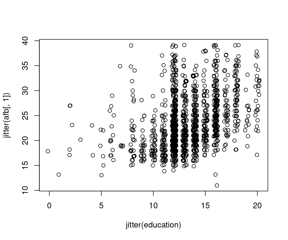
Example: Age at first birth (AFB) in US General Social Survey 2002. AFB is only known for women that have children. For women without children (but within child-bearing age) AFB is censored at their current age.

Load data and select subset:

data("GSS7402", package = "AER")
gss2002 <- subset(GSS7402,
  year == 2002 & (agefirstbirth < 40 | age < 40))

Compute censored AFB and declare censoring:

gss2002$afb <- with(gss2002, ifelse(kids > 0, agefirstbirth, age))
gss2002$afb <- with(gss2002, Surv(afb, kids > 0))

Observations now contain censoring information:

head(gss2002$afb)

## [1] 25+ 19  27  22  29  19+

Compute Kaplan-Meier estimator via survfit():

afb_km <- survfit(afb ~ 1, data = gss2002)
afb_skm <- summary(afb_km)
print(afb_skm)

## Call: survfit(formula = afb ~ 1, data = gss2002)
## 
##  time n.risk n.event survival  std.err lower 95% CI upper 95% CI
##    11   1371       1   0.9993 0.000729       0.9978       1.0000
##    13   1370       3   0.9971 0.001457       0.9942       0.9999
##    14   1367       2   0.9956 0.001783       0.9921       0.9991
##    15   1365      14   0.9854 0.003238       0.9791       0.9918
##    16   1351      40   0.9562 0.005525       0.9455       0.9671
##    17   1311      66   0.9081 0.007802       0.8929       0.9235
##    18   1245      97   0.8373 0.009967       0.8180       0.8571
##    19   1148     106   0.7600 0.011534       0.7378       0.7830
##    20   1030     122   0.6700 0.012726       0.6455       0.6954
##    21    898     123   0.5782 0.013406       0.5525       0.6051
##    22    767      97   0.5051 0.013612       0.4791       0.5325
##    23    654      72   0.4495 0.013600       0.4236       0.4770
##    24    563      61   0.4008 0.013480       0.3752       0.4281
##    25    484      60   0.3511 0.013248       0.3261       0.3781
##    26    407      45   0.3123 0.012986       0.2878       0.3388
##    27    351      45   0.2723 0.012618       0.2486       0.2981
##    28    294      37   0.2380 0.012223       0.2152       0.2632
##    29    246      32   0.2070 0.011795       0.1852       0.2315
##    30    209      38   0.1694 0.011119       0.1489       0.1926
##    31    163      18   0.1507 0.010730       0.1311       0.1733
##    32    135      19   0.1295 0.010264       0.1108       0.1512
##    33    108      17   0.1091 0.009766       0.0915       0.1300
##    34     83       7   0.0999 0.009542       0.0828       0.1205
##    35     65      13   0.0799 0.009101       0.0639       0.0999
##    36     45       7   0.0675 0.008815       0.0522       0.0872
##    37     29       7   0.0512 0.008572       0.0369       0.0711
##    38     17       3   0.0422 0.008499       0.0284       0.0626
##    39     12       2   0.0351 0.008411       0.0220       0.0562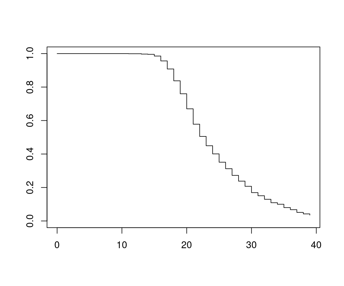

plot(afb_km, conf.int = FALSE)

with(afb_skm, plot(n.event/n.risk ~ time, type = "s"))

Remarks:

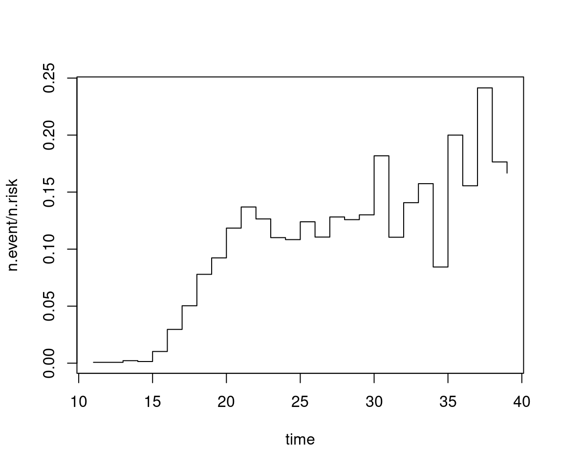
\(\hat h(t) = d_s / r_s\) for \(t_{(s)} \le t < t_{(s + 1)}\) is a less reliable estimator for the hazard function. Grouping or smoothing (similar to histograms or kernel densities) would be necessary but rare in practice.
Parametric approach: Estimate distribution parameters (and thus the associated survivor and hazard functions).
Moreover: Regression models are required that capture how survivor and hazard functions change with covariates.
Simple groupings can be incorporated nonparametrically in survfit(y ~ group).

Example: For data exploration, one could consider:

gss2002$edcat <- cut(gss2002$education, c(0, 12, 14, 20))
afb_km2 <- survfit(afb ~ edcat, data = gss2002)
plot(afb_km2, col = c(1, 2, 4))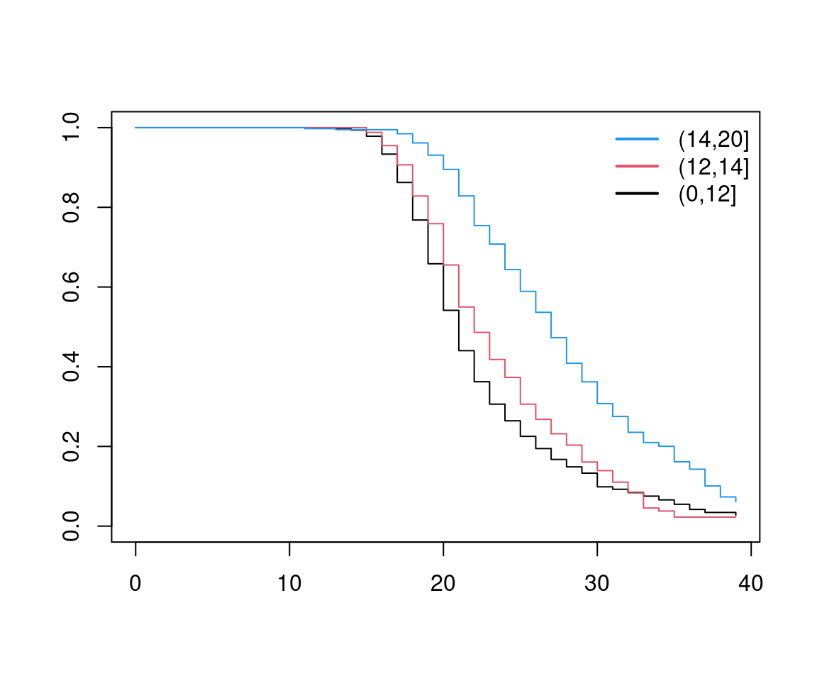

Observations: Survivor functions for different groups look very similar. This conveys that hazards are similar up to a factor. This is often exploited in modeling and inference.

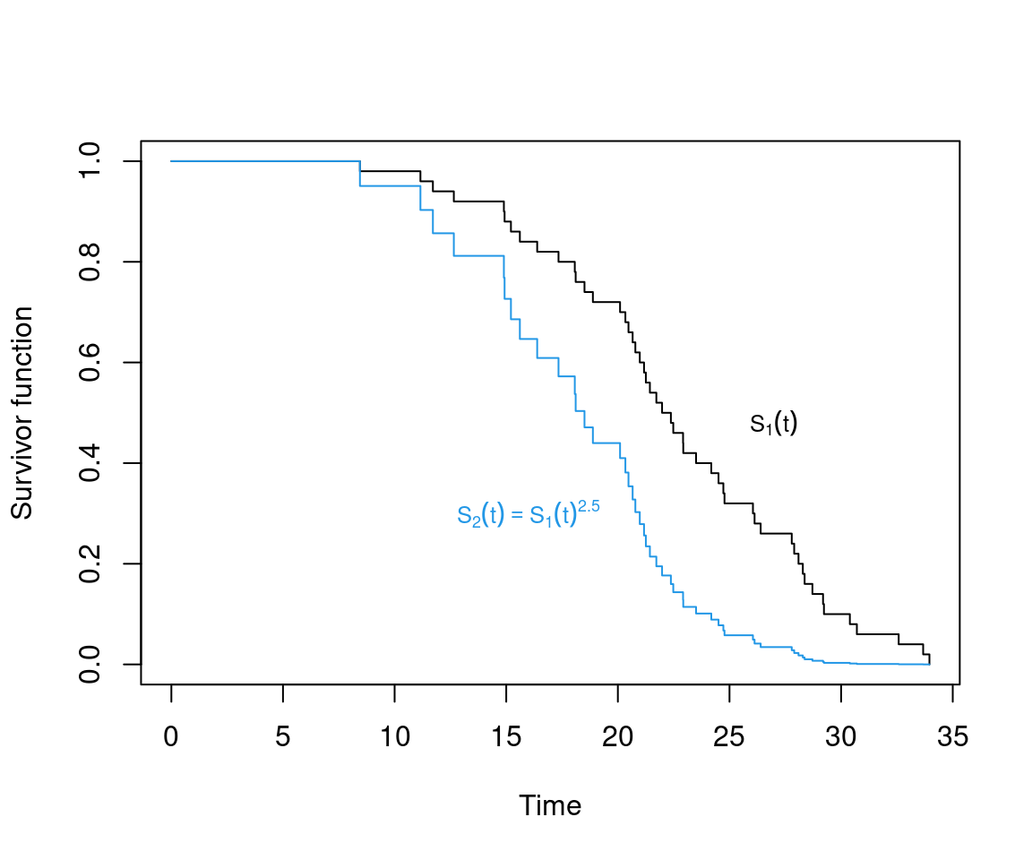
Formally: The assumption of proportional hazards for two groups entails

\[\begin{eqnarray*} h_2(t) & = & c \cdot h_1(t), \qquad \mbox{(or equivalently)}\\ S_2(t) & = & S_1(t)^c. \end{eqnarray*}\]

Implication: Survivor functions cannot cross.

Remark: Violations in practice are more serious for lower death/exit times (which are based on more observations).

9.3 Continuous Time Duration Models

Basic model: Constant hazard rate \(h(t) = \lambda\) (independent of duration \(t\)) is the simplest conceivable model for duration data.

Formally: Exponential distribution with hazard rate \(\lambda > 0\).

\[\begin{eqnarray*} f(t) & = & \lambda ~ \exp (- \lambda ~ t),\\ S(t) & = & \exp (- \lambda ~ t), \\ h(t) & = & \lambda. \end{eqnarray*}\]

Remarks:

Constant hazard rate is also called lack of memory.
In practice nonconstant hazards (depending on \(t\)) are relevant. In economics called duration dependence.

In R: d/p/q/rexp with parameter \(\mathtt{rate} = \lambda\).

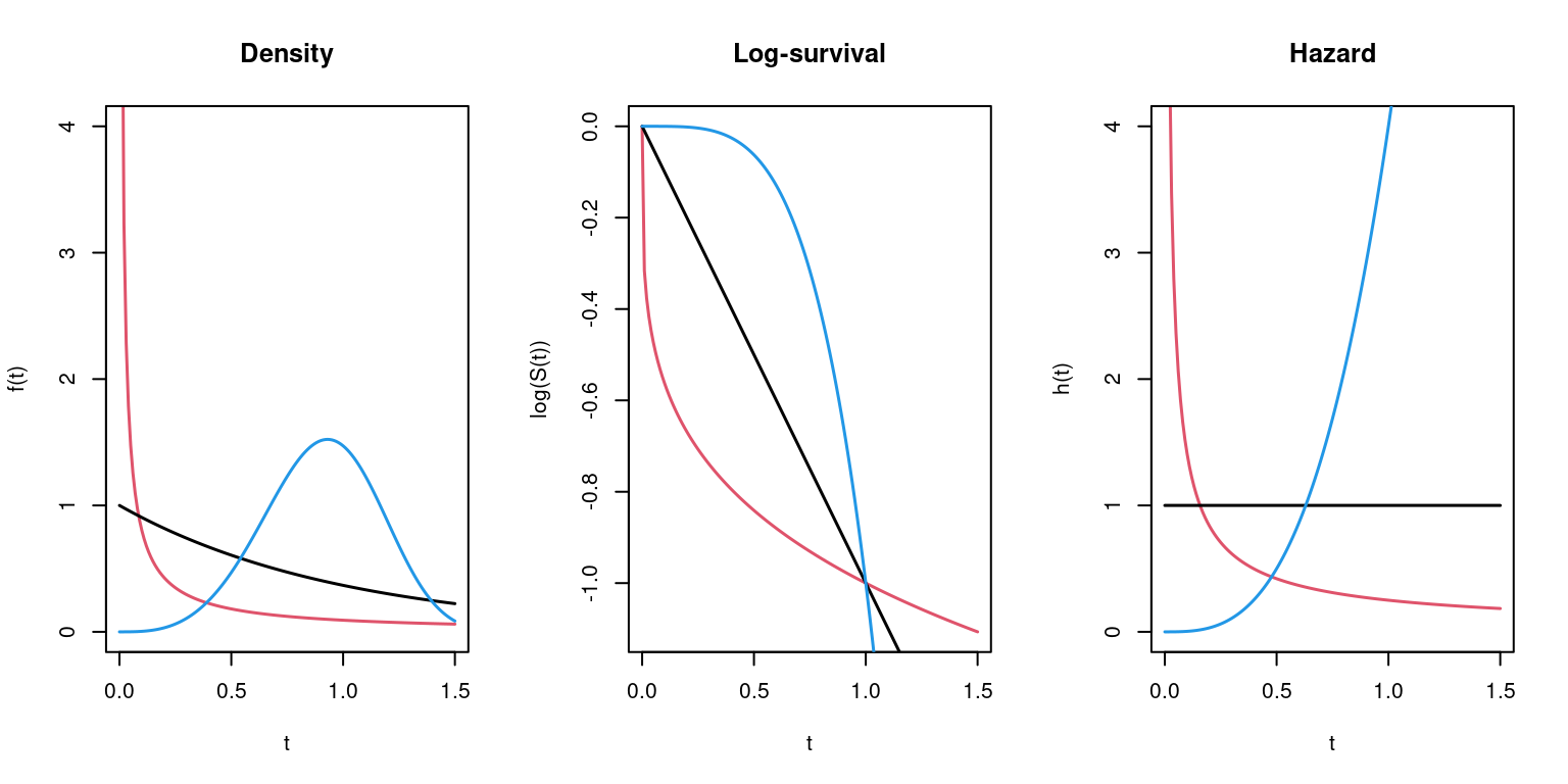
Generalization: Weibull distribution with additional shape parameter \(\alpha > 0\).

\[\begin{eqnarray*} f(t) & = & \lambda ~ \alpha ~ t^{\alpha - 1} ~ \exp (- \lambda ~ t^\alpha),\\ S(t) & = & \exp (- \lambda ~ t^\alpha), \\ h(t) & = & \lambda ~ \alpha ~ t^{\alpha - 1}. \end{eqnarray*}\]

Properties: The hazard function is always monotonic, for

\(\alpha > 1\) increasing,
\(\alpha = 1\) constant (exponential distribution),
\(\alpha < 1\) decreasing.

In R: d/p/q/rweibull with parameters \(\mathtt{scale} = \lambda^{-1/\alpha}\) and \(\mathtt{shape} = \alpha\). (Further parametrizations exist in the literature.)

Example: For \(\lambda = 1\) and \(\alpha = 1/4, 1, 4\).

Furthermore: Distributions with potentially non-monotonic hazard functions.

Lognormal distribution: \(\log(t) \sim \mathcal{N}(\mu, \sigma^2)\).
Loglogistic distribution.

9.4 Proportional Hazard Models

Idea: Assume proportional hazards for observations \(i = 1, \ldots, n\).

\[\begin{equation*} h_i(t) ~=~ \lambda_i \cdot h_0(t), \end{equation*}\]

where \(h_0(t)\) is called baseline hazard.

Regression: The factor \(\lambda_i\) is allowed to depend on a set of regressors \(x_i\), typically using a linear predictor and a log link.

\[\begin{equation*} \log(\lambda_i) ~=~ x_i^\top \beta. \end{equation*}\]

Thus: Baseline hazard corresponds to observation with \(x = 0\).

Parameter estimation: Two approaches for estimation of \(\beta\).

parametric: \(h_0(t, \alpha)\) parametric function,
semi-parametric: leave \(h_0(t)\) unspecified.

Parametric regression models: Most common models are

Exponential: \(h_0(t) = 1\).
Weibull: \(h_0(t) = \alpha ~ t^{\alpha - 1}\).

Inference: Via maximum likelihood, e.g., for exponential case.

\[\begin{eqnarray*} L(\beta) & = & \prod_{i = 1}^n \left\{\lambda_i \cdot \exp(- \lambda_i t_i)\right\}^{\delta_i} \exp(- \lambda_i t_i)^{1 - \delta_i} \\ & = & \prod_{i = 1}^n \lambda_i^{\delta_i} \exp(- \lambda_i t_i) \\ \log L(\beta) & = & \sum_{i = 1}^n \delta_i \cdot x_i^\top \beta - \sum_{i = 1}^n \exp(x_i^\top \beta) \cdot t_i, \end{eqnarray*}\]

where \(\delta_i = 1\) indicates an event and \(\delta_i = 0\) censoring.

In R: survreg() from package survival.

survreg(formula, data, subset, na.action, dist, ...)

with

formula: Response must be a "Surv" object from Surv().
dist: Distribution (implying link and variance functions etc.). Available distributions include "weibull" (default), "exponential", "logistic", "gaussian", "lognormal", "loglogistic".
Similar in spirit to GLMs. However, even without censoring not always special cases of exponential families.
Slightly different parametrization: Reports estimates for coefficients \(\tilde \beta\) and “scale” parameter \(\sigma\).
Corresponds to \(\beta = - \tilde \beta/\sigma\) in previous notation.
For Weibull: \(\alpha = 1/\sigma\).

Semiparametric regression: Cox proportional hazards model.

Idea: Maximum likelihood requires specification of the hazard, hence construct the conditional likelihood. Instead of \(\text{P}(T_i = t_i)\) use

\[\begin{equation*} \text{P}(T_i = t_i ~|~ \mbox{one event at } t_i). \end{equation*}\]

This leads to

\[\begin{equation*} \frac{h_0(t_i) \exp(x_i^\top \beta)}{\sum_{j: t_j \ge t_i} h_0(t_i) \exp(x_j^\top \beta)} ~=~ \frac{\exp(x_i^\top \beta)}{\sum_{j: t_j \ge t_i} \exp(x_j^\top \beta)} \end{equation*}\]

and thus, the conditional likelihood is

\[\begin{equation*} L(\beta) ~=~ \prod_{i = 1}^n \left(\frac{\exp(x_i^\top \beta)}{\sum_{j: t_j \ge t_i} \exp(x_j^\top \beta)}\right)^{\delta_i}. \end{equation*}\]

If there are censorings this is called {partial likelihood}.

In R: coxph() from survival.

Inference: For both parametric and semi-parametric models asymptotic normality can be shown. Hence, the usual inference (LR/Wald/score test, confidence intervals, information criteria) can be performed.

Interpretation: Similar to semi-logarithmic models. For observations \(x_1\) and \(x_2\)

\[\begin{equation*} \frac{h_1(t)}{h_2(t)} ~=~ \exp( (x_1 - x_2)^\top \beta), \end{equation*}\]

independent of \(t\).

Example: Determinants of AFB. Employ model formula

afb_f <- afb ~ education + siblings + ethnicity + immigrant + lowincome16 + city16

Of increased interest: influence of education.

afb_ex <- survreg(afb_f, data = gss2002, dist = "exponential")
afb_wb <- survreg(afb_f, data = gss2002, dist = "weibull")
modelsummary(list("AFB exponential" = afb_ex,
                  "AFB Weibull" = afb_wb), 
             fmt=3, estimate="{estimate}{stars}")

	AFB exponential	AFB Weibull
(Intercept)	2.707***	2.890***
	(0.170)	(0.037)
education	0.047***	0.026***
	(0.011)	(0.002)
siblings	−0.015	−0.007**
	(0.010)	(0.002)
ethnicitycauc	0.046	0.063***
	(0.072)	(0.016)
immigrantyes	0.094	0.034
	(0.093)	(0.021)
lowincome16yes	−0.027	0.007
	(0.074)	(0.017)
city16yes	0.037	0.026+
	(0.061)	(0.014)
Log(scale)		−1.487***
		(0.021)
Num.Obs.	1371	1371
AIC	9971.0	7688.7
BIC	10007.6	7730.5
RMSE	7.21	5.68

Comparison: Exponential and Weibull model can be compared using the standard likelihood methods.

lrtest(afb_ex, afb_wb)

## Likelihood ratio test
## 
## Model 1: afb ~ education + siblings + ethnicity + immigrant + lowincome16 + 
##     city16
## Model 2: afb ~ education + siblings + ethnicity + immigrant + lowincome16 + 
##     city16
##   #Df LogLik Df Chisq Pr(>Chisq)
## 1   7  -4979                    
## 2   8  -3836  1  2284     <2e-16

AIC(afb_ex, afb_wb)

##        df  AIC
## afb_ex  7 9971
## afb_wb  8 7689

afb_cph <- coxph(afb_f, data = gss2002)
coeftest(afb_cph)

## 
## z test of coefficients:
## 
##                Estimate Std. Error z value Pr(>|z|)
## education       -0.1138     0.0103  -11.04  < 2e-16
## siblings         0.0296     0.0103    2.86   0.0042
## ethnicitycauc   -0.2907     0.0730   -3.98  6.8e-05
## immigrantyes    -0.2011     0.0928   -2.17   0.0303
## lowincome16yes   0.0304     0.0742    0.41   0.6820
## city16yes       -0.0689     0.0607   -1.13   0.2564

Comparison: Parameter estimates.

cf <- cbind(
  "Exponential" = -coef(afb_ex),
  "Weibull" = -coef(afb_wb)/afb_wb$scale,
  "Cox-PH" = c(NA, coef(afb_cph))
)
cf

##                Exponential  Weibull   Cox-PH
## (Intercept)       -2.70684 -12.7815       NA
## education         -0.04679  -0.1133 -0.11380
## siblings           0.01549   0.0324  0.02961
## ethnicitycauc     -0.04560  -0.2800 -0.29069
## immigrantyes      -0.09401  -0.1517 -0.20108
## lowincome16yes     0.02725  -0.0310  0.03039
## city16yes         -0.03722  -0.1139 -0.06887

Hazard proportions:

exp(cf[-1,]) - 1

##                Exponential  Weibull   Cox-PH
## education         -0.04571 -0.10715 -0.10756
## siblings           0.01561  0.03293  0.03006
## ethnicitycauc     -0.04458 -0.24419 -0.25225
## immigrantyes      -0.08973 -0.14072 -0.18215
## lowincome16yes     0.02762 -0.03053  0.03086
## city16yes         -0.03654 -0.10765 -0.06655

Compare survivor functions at \(\bar x\):

xbar <- colMeans(model.matrix(afb_ex, data = gss2002))

Distribution parameters:

lambda_ex <- exp(c(- xbar %*% coef(afb_ex)))
lambda_wb <- exp(c(- xbar %*% coef(afb_wb)) / afb_wb$scale)
alpha_wb <- 1/afb_wb$scale

Visualization (using Kaplan-Meier at \(\bar x\) for Cox-PH):

plot(afb_km, conf.int = FALSE)
tt <- 0:400/10
lines(tt, exp(-lambda_ex * tt), col = 3)
lines(tt, exp(-lambda_wb * tt^alpha_wb), col = 4)
lines(survfit(afb_cph), col = 2)

Alternatively: Using R’s own exponential and Weibull functions requires reparametrization, i.e.

pexp(tt, rate = lambda_ex, lower.tail = FALSE)
pweibull(tt, scale = lambda_wb^(-1/alpha_wb), shape = alpha, lower.tail = FALSE)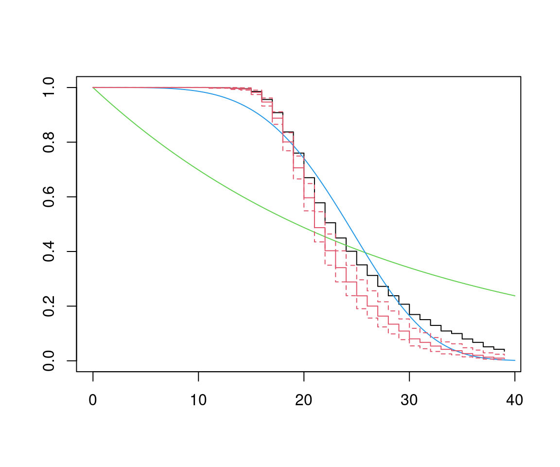

Conclusions:

Exponential is clearly inappropriate.
Weibull and Cox-PH lead to similar results.
Cox-PH has least restrictive assumptions.

9.5 Outlook

Alternative models: Instead of proportional hazards (PH) models, employ accelerated failure time (AFT) models.

\[\begin{equation*} \log(t_i) ~=~ x_i^\top \beta ~+~ \varepsilon_i, \end{equation*}\]

e.g., leading to lognormal model (if \(\varepsilon\) is normal) or loglogistic model (if \(\varepsilon\) is logistic).

Failure time acceleration can be seen via reparametrization

\[\begin{equation*} \log(\psi_i \cdot t_i) ~=~ \varepsilon_i, \end{equation*}\]

with \(\psi_i = \exp(- x_i^\top \beta)\) leading to shortened/lengthened survival times for \(\psi_i > 1\) and \(\psi_i < 1\), respectively.

Weibull/exponential model is the only model that is both of AFT and PH type.

Unobserved heterogeneity: Account for via additional random effects. In duration analysis called frailty models. Example: Exponential duration with gamma frailty

\[\begin{equation*} \lambda_i ~=~ \nu \cdot \exp(x_i^\top \beta), \end{equation*}\]

where \(\nu \sim \mathit{Gamma}(\theta, \theta)\) leading to Pareto type~II distribution.

Further extensions:

Need to incorporate time-varying regressors \(x_{it}\).
Competing risks: Deaths/exits can be caused by different types of events.
Example: Unemployment can be terminated by job or withdrawal from labor market.