Chapter 5 Multinomial Response Models

5.1 Introduction

In this chapter, we study probability models for analyzing multinomial data. Multinomial variables have three or more possible outcomes that are nominal (unordered), mutually exclusive categories. Typical economic examples for multinomial responses include:

• Employment status.
  \(y_i\): Person \(i\) works, unemployed, not in labor force.
  Potential covariates: Education, work experience, …
• Party preferences.
  \(y_i\): Voter \(i\) votes conservative, social, liberal, green, …
  Potential covariates: Age, gender, occupation, …
• Travel mode choice.
  \(y_i\): Person \(i\) travels to work via airplane, train, bus, car.
  Potential subject covariates: Income, distance, …
  Potential alternative covariates: Price, travel time, …
• Brand choice.
  \(y_i\): Person \(i\) chooses good of brand A, B, C, D, …
  Potential subject covariates: Income, marital status, …
  Potential alternative covariates: Price, advertising, …

A multinomial dependent variable \(y_i\) has \(m\) unordered mutually exclusive outcomes \(j = 1, \dots, m\) (without loss of generality). For example, an individual can fall into one of \(m=3\) categories regarding their employment status: employed, unemployed, or out of the labor force. Our goal is to model the corresponding occurrence probabilities of the outcomes, given the covariates. The covariates can be an individual-specific set of regressors \(x_i\) and/or alternative-specific regressors \(z_{ij}\). When modeling travel mode choice, for example, a possible individual-specific regressor is the distance one needs to travel from home to work, while a possible alternative-specific regressor could be the price of a bus ticket, or the length of the bus ride.

\[\begin{equation*} \pi_{ij} ~=~ \text{P}(y_i = j ~|~ x_i, z_{ij}). \end{equation*}\]

Since the \(m\) categories are mutually exclusive and collectively exhaustive, the occurrence probabilities of each outcome are necessarily between 0 and 1 (\(0 ~\le~ \pi_{ij} ~\le~ 1\)), and the corresponding probabilities for each category sum up to one \(\sum_{j = 1}^m \pi_{ij} = 1\) for all \(i = 1, \dots, n\). Furthermore, all parameters must be identified, which means we can have a maximum of \(m-1\) coefficients that compare the probability of an outcome (category) to the probability of a so-called base category.

First, we take a quick excursion to introduce the multinomial distribution. The multinomial distribution is a discrete multivariate distribution, which is a generalization of the binomial (and thus Bernoulli) distribution. The setup is the following: there are \(N\) independently identically distributed (i.i.d.) experiments which lead to one of \(m\) mutually exclusive outcomes \(A_1, \dots, A_m\). Let \(Y_l = (Y_{1l}, \dots, Y_{ml})\) vector-valued indicators

\[\begin{equation*} Y_{jl} ~=~ \left\{ \begin{array}{ll} 1 & \mbox{if $A_j$ is observed in $l$-th experiment,}\\ 0 & \mbox{otherwise.} \end{array} \right. \end{equation*}\]

Where by construction, \(\sum_{j = 1}^m Y_{jl} = 1\), and \(Y_{jl}\) and \(Y_{kl}\) are dependent. Let \(X = (X_1, \dots, X_m)\) with \(X_j = \sum_{l = 1}^N Y_{jl}\), i.e., the number of observations of \(A_j\) in \(N\) trials. In particular, \(\sum_{j = 1}^m X_j = N\). We denote the multinomially distributed variable \(X\) with N trials and \(m\) possible outcomes with their corresponding occurrence probabilities by \(X \sim \mathit{MN}(N, \pi_1, \dots, \pi_m)\). The probability density function for \(x_j \in \{0, 1, \dots, N\}\) and \(\sum_{j = 1}^m x_j = N\) is

\[\begin{eqnarray*} f(x) ~=~ f(x_1, \dots, x_m) & = & \text{P}(X_1 = x_1, \dots, X_m = x_m) \\ & = & \frac{N!}{x_1! \cdots x_m!} \prod_{j = 1}^m \pi_j^{x_j}. \end{eqnarray*}\]

Special cases of the multivariate distribution are the binomial distribution \(\mathit{Bin}(N, \pi)\) for \(m = 2\), using w.l.o.g. \(\pi = \pi_2\) and \(\pi_1 = 1 - \pi_2\); and the Bernoulli distribution, where we additionally have the number of trials \(N = 1\). Subsequently, we are going to analyze models with \(N = 1\), i.e., a single experiment with \(m\) possible outcomes. (Note: In case there are more trials, these should be independent: the same person cannot be asked on different days, for example. For \(N \geq 2\) trials, aggregated data can be used, as there is usually not much correlation between individual trials in this case.) A novelty of this model is that the expected value \(\text{E}(X)\) is not of interest, only the parameters \(\pi_1, \dots, \pi_m\).

5.2 Multinomial Logit Model

The multinomial logit model is the simplest among multinomial response models. The idea is to have a response variable \(Y_i\) with \(i = 1, \dots, n\) independent observations: \(Y_i \sim \mathit{MN}(1, \pi_{i1}, \dots, \pi_{im})\). Initially, we only consider individual-specific regressors \(x_i\) as covariates. We denote the outcome by \(y_i \in \{1, \dots, m\}\) for each \(i = 1, \dots, n\) and the corresponding binary indicators by \(d_{ij} \in \{0, 1\}\) for each \(j = 1, \dots, m\) category, where

\[\begin{equation*} d_{ij} ~=~ \left\{ \begin{array}{ll} 1 & \mbox{if $y_i = j$,}\\ 0 & \mbox{otherwise.} \end{array} \right. \end{equation*}\]

The joint distribution of the multinomial probability function is

\[\begin{equation*} f(y_i ~|~ x_i) ~=~ \pi_{i1}^{d_{i1}} \cdots \pi_{im}^{d_{im}} ~=~ \prod_{j = 1}^m \pi_{ij}^{d_{ij}}, \end{equation*}\]

with \(\sum_{j = 1}^m \pi_{ij} = 1\) and \(\sum_{j = 1}^m d_{ij} = 1\) for \(i = 1, \dots, n\).

Due to the constraint that \(\pi_{ij}\) sum up to one, we reparameterize (without loss of generality):

\[\begin{equation*} \pi_{i1} ~=~ 1 ~-~ \sum_{j = 2}^m \pi_{ij}. \end{equation*}\]

To link the regressors \(x_i\) with the parameters \(\pi_i\), we use a linear predictor \(\eta_{ij}\) based on alternative-specific coefficients \(\beta_j\). Then, we link the linear predictor to log-odds (most typical link function). Recall that log-odds in binomial models correspond to success/failure probability. In the multinomial model, log-odds are the success probability of category \(j\) in comparison with the success probability of category \(1\), i.e., the success probability with respect to a reference category.

\[\begin{equation*} \log \left( \frac{\pi_{ij}}{\pi_{i1}} \right) ~=~ \eta_{ij} ~=~ x_i^\top \beta_j, \end{equation*}\] for \(j = 2, \dots, m\).

This implies:

\[\begin{eqnarray*} \pi_{ij} & = & \exp(\eta_{ij}) \cdot \pi_{i1} \qquad (j = 2, \dots, m), \\ \pi_{i1} & = & 1 - \sum_{s = 2}^m \exp(\eta_{is}) \cdot \pi_{i1}, \end{eqnarray*}\]

which is equivalent to

\[\begin{eqnarray*} \pi_{ij} & = & \frac{\exp(x_i^\top \beta_j)}{1 + \sum_{s = 2}^m \exp(x_i^\top \beta_s)} \qquad (j = 2, \dots, m), \\ \pi_{i1} & = & \frac{1}{1 + \sum_{s = 2}^m \exp(x_i^\top \beta_s)}. \\ \end{eqnarray*}\]

Somewhat more compactly, the multinomial logit model (MNL) can be written as:

\[\begin{equation*} \pi_{ij} ~=~ \frac{\exp(x_i^\top \beta_j)}{\sum_{s = 1}^m \exp(x_i^\top \beta_s)}, \end{equation*}\]

for \(j = 1, \dots, m\) using \(\beta_1 \equiv 0\) as the identification restriction, making category \(1\) the reference category. Note that the reference category is arbitrarily chosen, so that any other \(\beta_j\) could be set to zero.

The multinomial logit model is a multiple index model for \(m > 2\). As mentioned earlier, we do not model the conditional mean, as it is not meaningful in case of multinomially distributed variables. Remember, furthermore, that all parameters \(\pi_{ij}\) are in relation to the reference category.

To estimate the model, we derive the likelihood, the log-likelihood, and the score function.

\[\begin{eqnarray*} L(\beta_2, \dots, \beta_m; y, x) & = & \prod_{i = 1}^n f(y_i ~|~ x_i; \beta_2, \dots, \beta_m) ~=~ \prod_{i = 1}^n \prod_{j = 1}^m \pi_{ij}^{d_{ij}} \\ \ell(\beta_2, \dots, \beta_m) & = & \sum_{i = 1}^n \sum_{j = 1}^m d_{ij} \cdot \log(\pi_{ij}) \qquad (\le 0) \\ \frac{\partial \ell}{\partial \beta_s} & = & \sum_{i = 1}^n \sum_{j = 1}^m d_{ij} \frac{1}{\pi_{ij}} \frac{\partial \pi_{ij}}{\partial \beta_s} \qquad (s = 2, \dots, m) \\ \frac{\partial \pi_{ij}}{\partial \beta_s} & = & \left\{ \begin{array}{ll} -\pi_{ij} ~ \pi_{is} ~ x_i & s \neq j \\ \pi_{is} ~ (1 - \pi_{is}) ~ x_i & s = j \end{array} \right. \end{eqnarray*}\]

For the score, as \(d_{is} \cdot \pi_{is} + \sum_{j \neq s} d_{ij} \cdot \pi_{is} = \pi_{is}\), one can write

\[\begin{eqnarray*} \frac{\partial \ell}{\partial \beta_s} & = & \sum_{i = 1}^n \left( d_{ij} ~ (1 - \pi_{is}) ~ x_i ~+~ \sum_{j \neq s} -d_{ij} ~ \pi_{is} ~ x_i \right) \\ & = & \sum_{i = 1}^n (d_{is} - \pi_{is}) ~ x_i \qquad (s = 2, \dots, m). \end{eqnarray*}\]

The corresponding Hessian matrix is

\[\begin{eqnarray*} \frac{\partial^2 \ell}{\partial \beta_s \partial \beta_s^\top} & = & - \sum_{i = 1}^n \pi_{is} ~ (1 - \pi_{is}) ~ x_i x_i^\top,\\ \frac{\partial^2 \ell}{\partial \beta_s \partial \beta_t^\top} & = & \sum_{i = 1}^n \pi_{is} ~ \pi_{it} ~ x_i x_i^\top. \end{eqnarray*}\]

It can be shown that the problem is “well-behaved”: the Hessian is negative definite, which means the likelihood function is globally concave (and bounded), ensuring uniqueness of maximum. Moreover, if the model is correctly specified, the maximum likelihood estimator is consistent, efficient, and asymptotically normally distributed. We can also see that the Hessian does not depend on \(y_{ij}\) or \(d_{ij}\), which means in its actual value is equal to its expected value, \(I = J\). Note, however, that maximum likelihood estimation for multinomial models is much more complicated than for binomial logit/probit, because each individual probability \(\pi_{ij}\) depends on all coefficients \(\beta_j\), and thus the cross-derivatives are non-zero, which means the Hessian is not block-diagonal, and MLE can not be derived from “dichotomized” logit models.

5.2.1 Example: Bank wages

As an example, we examine cross-section data on job categories of employees of a US bank. We use a data frame containing 474 observations on 4 variables:

Table 5.1: Variables in the Bank Wages Data Set

Variable	Description
job	Job category with levels "custodial", "admin", and "manage"
education	Education in years.
gender	Gender.
minority	Is the employee member of a minority?

data("BankWages", package = "AER")
summary(BankWages)

##         job        education       gender    minority 
##  custodial: 27   Min.   : 8.0   male  :258   no :370  
##  admin    :363   1st Qu.:12.0   female:216   yes:104  
##  manage   : 84   Median :12.0                         
##                  Mean   :13.5                         
##                  3rd Qu.:15.0                         
##                  Max.   :21.0

xtabs(~ job + education, data = BankWages)

##            education
## job           8  12  14  15  16  17  18  19  20  21
##   custodial  13  13   0   1   0   0   0   0   0   0
##   admin      40 176   6 111  24   3   2   1   0   0
##   manage      0   1   0   4  35   8   7  26   2   1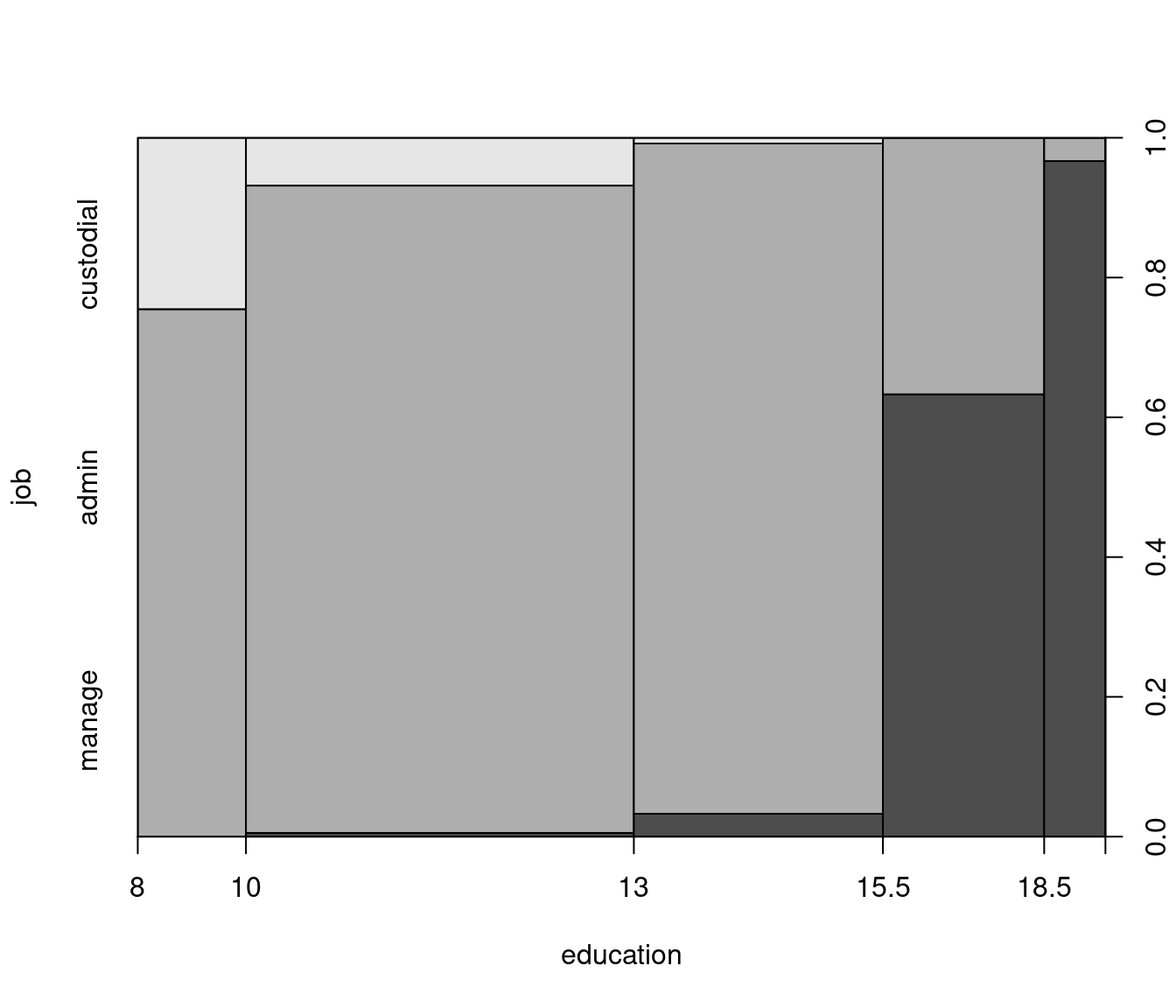

plot(job ~ education, data = BankWages,
  breaks = c(8, 10, 13, 15.5, 18.5, 21))

Figure 5.1: Job Category Plotted Against Education

For further exploratory analysis only, we split education into categories, in order to create contingency tables and spine plots for visualization:

BankWages$edcat <- factor(BankWages$education)
levels(BankWages$edcat)[3:10] <- rep(c("14-15", "16-18", "19-21"),
  c(2, 3, 3))

We can then create a four-way table of all variables (with new education categories) and display the “flat” version of the table via ftable(), with edcat as main “explanatory” variable and job as main “dependent” variable. We also use gender and minority for nesting. To visualize the data, create a nested spinogram via mosaicplot(), again for job by edcat, and nesting in gender and minority - be aware that the sequence of splitting variables matters for visualization in mosaic plots.

Note: mosaicplot() is available in base R. For more flexible visualization, we can also use the vcd package’s mosaic() and doubledecker() functions, where the latter creates vertical splits only.

bw_tab <- xtabs(~ gender + minority + edcat + job,
  data = BankWages)
ftable(bw_tab, col.vars = "edcat")

##                           edcat   8  12 14-15 16-18 19-21
## gender minority job                                      
## male   no       custodial         6   8     0     0     0
##                 admin             6  30    66     7     1
##                 manage            0   0     4    38    28
##        yes      custodial         7   5     1     0     0
##                 admin             4  18    18     7     0
##                 manage            0   1     0     2     1
## female no       custodial         0   0     0     0     0
##                 admin            27 101    25    13     0
##                 manage            0   0     0    10     0
##        yes      custodial         0   0     0     0     0
##                 admin             3  27     8     2     0
##                 manage            0   0     0     0     0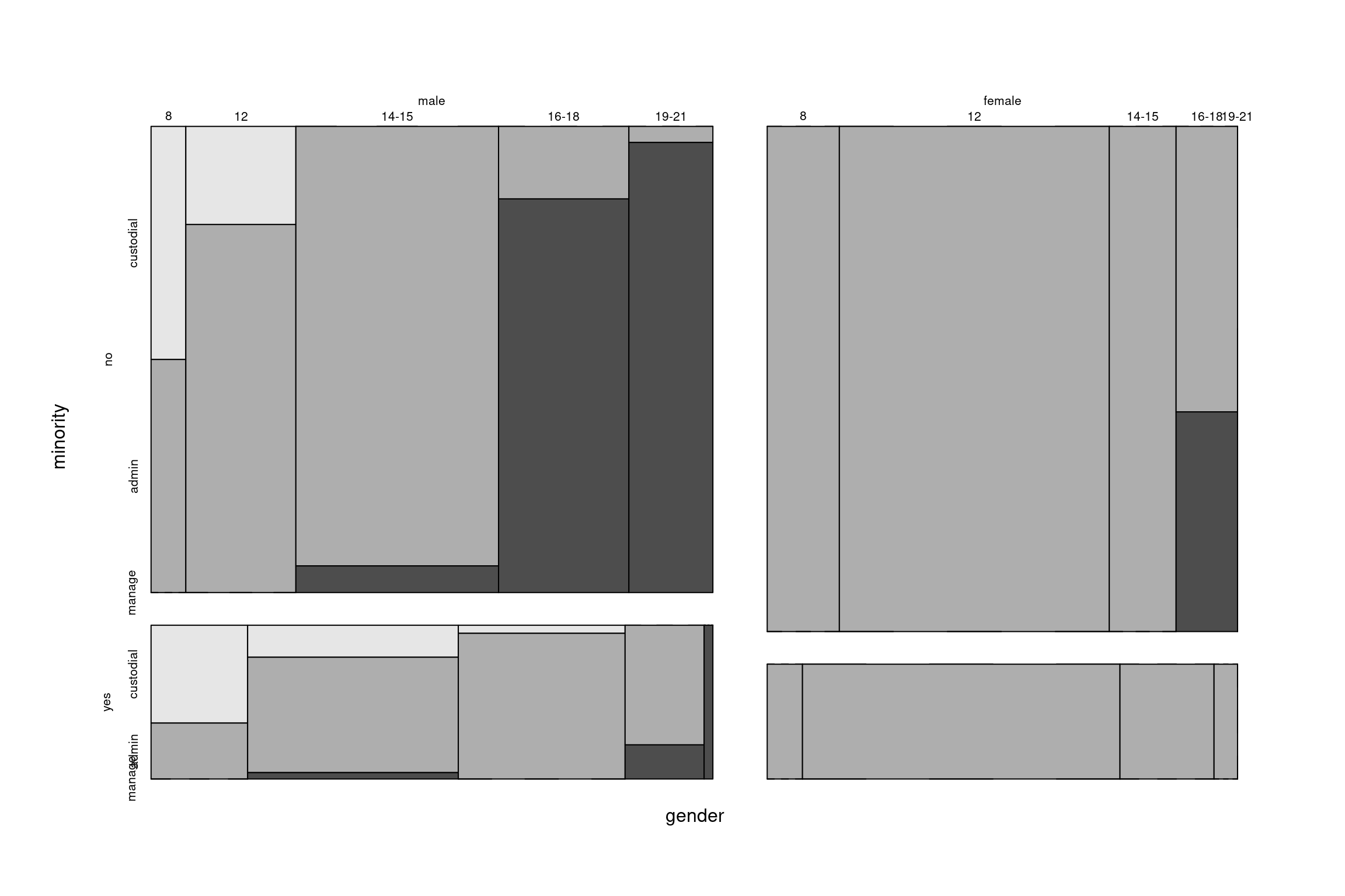

mosaicplot(bw_tab, off = c(5, 5, 0, 0),
  col = rev(gray.colors(3)), main = "")

Figure 5.2: Mosaic Plot of the Bank Wages Data

5.2.2 Bank wages: Estimation

To illustrate estimation with an example, we fit a multinomial logit model with two regressors. As the sample does not include any females working in custodial services, and only few in management, there is not much we can learn from the female data, and therefore we turn our attention to analyzing the subsample of males. In R, this is implemented with the multinom() function in package nnet (accompanying Venables & Ripley 2002), which uses the same fitting algorithm as for artificial neural networks. Note: the trace=FALSE setting is responsible for omitting the detailed likelihood calculation.

library("nnet")
bwmale <- subset(BankWages, gender == "male")
(bw_mnl <- multinom(job ~ education + minority,
  data = bwmale, trace = FALSE))

## Call:
## multinom(formula = job ~ education + minority, data = bwmale, 
##     trace = FALSE)
## 
## Coefficients:
##        (Intercept) education minorityyes
## admin       -4.761    0.5534     -0.4269
## manage     -30.775    2.1868     -2.5360
## 
## Residual Deviance: 237.5 
## AIC: 249.5

Reference category is by default the first one, here "custodial".

summary(bw_mnl)

## Call:
## multinom(formula = job ~ education + minority, data = bwmale, 
##     trace = FALSE)
## 
## Coefficients:
##        (Intercept) education minorityyes
## admin       -4.761    0.5534     -0.4269
## manage     -30.775    2.1868     -2.5360
## 
## Std. Errors:
##        (Intercept) education minorityyes
## admin        1.173   0.09904      0.5027
## manage       4.479   0.29484      0.9342
## 
## Residual Deviance: 237.5 
## AIC: 249.5

coeftest(bw_mnl)

## 
## z test of coefficients:
## 
##                    Estimate Std. Error z value Pr(>|z|)
## admin:(Intercept)    -4.761      1.173   -4.06  4.9e-05
## admin:education       0.553      0.099    5.59  2.3e-08
## admin:minorityyes    -0.427      0.503   -0.85   0.3957
## manage:(Intercept)  -30.775      4.479   -6.87  6.4e-12
## manage:education      2.187      0.295    7.42  1.2e-13
## manage:minorityyes   -2.536      0.934   -2.71   0.0066

5.2.3 Bank wages: Inference

The lrtest() function can be used for likelihood ratio tests between nested models. As an example, we assess the joint significance of all minority effects.

bw_mnl1 <- multinom(job ~ education, data = bwmale, trace = FALSE)
lrtest(bw_mnl, bw_mnl1)

## Likelihood ratio test
## 
## Model 1: job ~ education + minority
## Model 2: job ~ education
##   #Df LogLik Df Chisq Pr(>Chisq)
## 1   6   -119                    
## 2   4   -124 -2  10.4     0.0055

Note that the function waldtest() does not work for "multinom" objects, yet. (To be fixed.)

5.2.4 Interpretation of parameters

The interpretation of parameters of multinomial models is based on similar ideas as we have seen with the binomial logit model. One option is to assess the influence of a given regressor in terms of probabilities, either by calculating the individual probabilities (i.e., effects) or investigating their partial changes (i.e., marginal effects). Alternatively, we can assess odds, or odds ratios. The important difference to binomial models is that in multinomial models, all coefficients \(\beta_j\) need to be interpreted relative to the base category.

The odds of alternative \(j\) against reference category \(1\) or arbitrary alternative \(s\) are

\[\begin{eqnarray*} \frac{\pi_{ij}}{\pi_{i1}} & = & \exp(x_i^\top \beta_j) \qquad (j = 2, \dots, m), \\ \frac{\pi_{ij}}{\pi_{is}} & = & \exp(x_i^\top (\beta_j - \beta_s)) \qquad (j, s = 2, \dots, m). \end{eqnarray*}\]

The odds ratios, to compare two (groups of) subjects, are

\[\begin{eqnarray*} \frac{\pi_{aj}/\pi_{a1}}{\pi_{bj}/\pi_{b1}} & = & \exp((x_a - x_b)^\top \beta_j), \\ \frac{\pi_{aj}/\pi_{as}}{\pi_{bj}/\pi_{bs}} & = & \exp((x_a - x_b)^\top (\beta_j - \beta_s)). \end{eqnarray*}\]

A special case of this is when \(x_a = x_b + \Delta x_{bl}\) differ only for the \(l\)-th regressor by one unit \(\Delta x_{bl} = (0, \dots, 1, \dots, 0)^\top\), i.e., we only change one of the regressors by one unit, while everything else remains equal:

\[\begin{eqnarray*} \frac{\pi_{aj}/\pi_{a1}}{\pi_{bj}/\pi_{b1}} & = & \exp(\Delta x_{bl} \cdot \beta_l) ~=~ \exp(\beta_{jl}), \\ \frac{\pi_{aj}/\pi_{as}}{\pi_{bj}/\pi_{bs}} & = & \exp(\Delta x_{bl} \cdot (\beta_j - \beta_s)) ~=~ \exp(\beta_{jl} - \beta_{sl}). \end{eqnarray*}\]

Relative increases/decreases in odds ratios by single-unit changes in regressors are thus captured in coefficients or their differences. For “small” values, (differences of) coefficients can be directly interpreted.

\[\begin{eqnarray*} \frac{\pi_{aj}/\pi_{a1}}{\pi_{bj}/\pi_{b1}} ~-~ 1 & = & \exp(\beta_{jl}) ~-~ 1 ~\approx~ \beta_{jl}, \\ \frac{\pi_{aj}/\pi_{as}}{\pi_{bj}/\pi_{bs}} ~-~ 1 & = & \exp(\beta_{jl} - \beta_{sl}) ~-~ 1 ~\approx~ \beta_{jl} - \beta_{sl}. \end{eqnarray*}\]

An example: Choice between means of transport, where the alternatives are car (1), bus (2), and train (3). Suppose that

\[\begin{equation*} \frac{\pi_2}{\pi_1} ~=~ \frac{3}{4}, \qquad \frac{\pi_3}{\pi_1} ~=~ \frac{3}{4}. \end{equation*}\]

This implies \(\pi_1 = (1 + 3/4 + 3/4)^{-1} = 0.4\) and thus:

\[\begin{equation*} \pi_2 ~=~ 0.3, \qquad \pi_3 ~=~ 0.3. \end{equation*}\]

Suppose that there is a single-unit change in the \(l\)-th regressor with the following coefficients:

\[\begin{equation*} \begin{array}{rclcrcl} \beta_{2l} & = & -0.2231 && \beta_{3l} & = & -0.6286 \\ \exp(\beta_{2l}) & = & 4/5 && \exp(\beta_{3l}) & = & 8/15 \\ \frac{\pi'_2/\pi'_1}{\pi_2/\pi_1} & = & 4/5 && \frac{\pi'_3/\pi'_1}{\pi_3/\pi_1} & = & 8/15 \\ \pi'_2/\pi'_1 & = & 3/5 && \pi'_3/\pi'_1 & = & 2/5 \\ \pi'_2 & = & 0.3 && \pi'_3 & = & 0.2 \end{array} \end{equation*}\]

and \(\pi'_1 = (1 + 3/5 + 2/5)^{-1} = 0.5\).

To conclude: the sign of a coefficient does not even determine the sign of change in probability! In this example, \(\beta_{2l}\) is negative, but \(\pi_2\) does not change, only the odds compared to the reference category do. In our previous bank example, an increase in the odds (i.e., a positive coefficient) \(\frac{\pi_{admin}}{\pi_{custodial}}\) may be due to an increase in \(\pi_{admin}\), or a decrease in \(\pi_{custodial}\), or both. It is even possible that both \(\pi_{admin}\) and \(\pi_{custodial}\) are increasing, and \(\pi_{admin}\) increases faster. Thus, the direction of change in individual probabilities is not as clear as we have seen it in the binomial model, as probabilities and effects for alternative \(j\) depend on parameters for all alternatives \(j = 1, \dots, m\).

The marginal probability effects (MPE) are:

\[\begin{eqnarray*} \mathit{MPE}_{i1l} & = & \frac{\partial \pi_{i1}}{\partial x_{il}} ~=~ - \pi_{i1} \sum_{s = 2}^m \pi_{is} \beta_{sl}, \\ \mathit{MPE}_{ijl} & = & \frac{\partial \pi_{ij}}{\partial x_{il}} ~=~ \pi_{ij} \left(\beta_{jl} ~-~ \sum_{s = 2}^m \pi_{is} \beta_{sl} \right) \qquad (j = 2, \dots, m).\\ \end{eqnarray*}\]

For the average marginal probability effects (AMPE), evaluate and average at \(\hat \beta_2, \dots, \hat \beta_m\).:

\[\begin{equation*} \widehat{\mathit{AMPE}}_{jl} ~=~ \frac{1}{n} \sum_{i = 1}^n \widehat{\mathit{MPE}}_{ijl} \qquad (j = 1, \dots, m). \end{equation*}\]

Discrete changes are somewhat easier to interpret.:

\[\begin{equation*} \Delta \pi_{ij} ~=~ \text{Prob}(y_i = j ~|~ x_i + \Delta x_{il}) ~-~ \text{Prob}(y_i = j ~|~ x_i) \qquad (j = 1, \dots, m), \end{equation*}\]

where \(x_i\) is often chosen as the average regressor \(\bar x\).

5.2.5 Bank wages: Effects

As a next step in our bank wages example, we visualize the probability effects at \(\bar x\) while changing only the \(l\)-th regressor. In particular, we plot \(\Delta \bar x_{l}\) against \(\text{Prob}(y_i = j ~|~ \bar x + \Delta \bar x_{l})\). First, compute all effects for MNL model for BankWages data.

library("effects")
bw_eff <- allEffects(bw_mnl, xlevels = list(education = 50))

We can plot education and minority effects in three different ways:

plot(bw_eff)

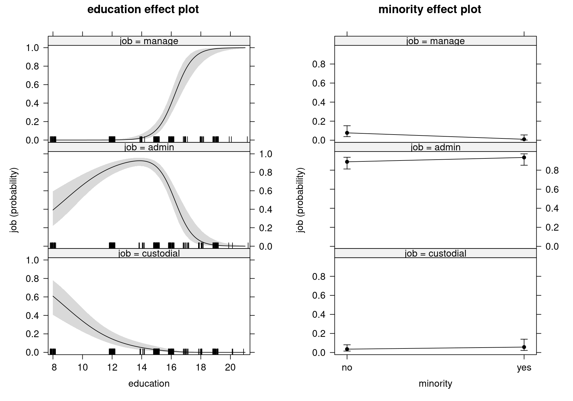
Figure 5.3: Education and Minority Effects on Job Categories: Separate Probability Curves with Pointwise Confidence Bands

plot(bw_eff, multiline = TRUE, colors = c(1, 2, 4))

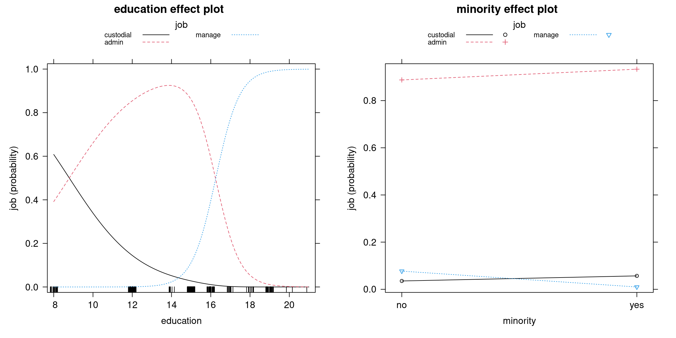
Figure 5.4: Education and Minority Effects: Probability Curves in a Single Display

plot(bw_eff, style = "stacked", colors = gray.colors(3))

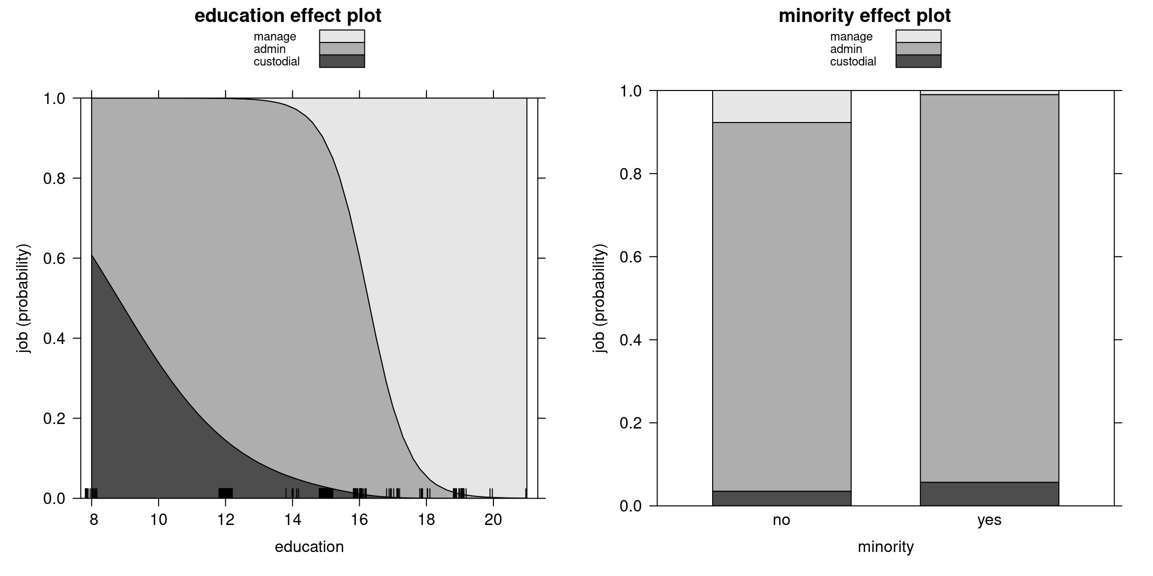
Figure 5.5: Education and Minority Effects: Cumulative Probability Curves in a Single Display

5.2.6 Bank wages: Goodness of fit

To assess the model’s goodness of fit, we can create a confusion matrix (observed vs. predicted values):

xtabs(~ job + predict(bw_mnl, type = "class"), data = bwmale)

##            predict(bw_mnl, type = "class")
## job         custodial admin manage
##   custodial        13    14      0
##   admin            10   138      9
##   manage            0     7     67

where the predicted category is

\[\begin{equation*} \hat y_i ~=~ \underset{j = 1, \dots, m}{argmax}\: \hat \pi_{ij}. \end{equation*}\]

Alternatively, we can assess goodness of fit with the McFadden \(R^2\) is (as seen in Chapter 4):

1 - as.vector(logLik(bw_mnl) / logLik(update(bw_mnl, . ~ 1)))

## [1] 0.4868

5.2.7 Bank wages: Other R packages

R offers various implementations: MNL can be estimated by several functions.

• nnet: multinom() is the reference implementation. Other packages cooperate with this, e.g., effects or lmtest (lrtest(),coeftest()).
• VGAM: vglm() estimates vector GLMs and GAMs (generalized additive models). Very wide and flexible class of models, however, its methods interface is somewhat nonstandard.
• mlogit: mlogit() estimates a wide variety of flavors of multinomial response models. Cooperates with lmtest (but not effects). More details later.

Package VGAM: Default reference category is \(m\) (not 1).

library("VGAM")
bwmale2 <- bwmale

bwmale2$job <- factor(bwmale2$job,
  levels = c("admin", "manage", "custodial"), ordered = FALSE)
bw_vglm <- vglm(job ~ education + minority, family = multinomial,
  data = bwmale2)
coef(bw_vglm, matrix = TRUE)

##             log(mu[,1]/mu[,3]) log(mu[,2]/mu[,3])
## (Intercept)            -4.7607            -30.775
## education               0.5534              2.187
## minorityyes            -0.4270             -2.536

summary(bw_vglm)

## 
## Call:
## vglm(formula = job ~ education + minority, family = multinomial, 
##     data = bwmale2)
## 
## Coefficients: 
##               Estimate Std. Error z value Pr(>|z|)
## (Intercept):1   -4.761      1.173   -4.06  4.9e-05
## (Intercept):2  -30.775      4.479   -6.87  6.4e-12
## education:1      0.553      0.099    5.59  2.3e-08
## education:2      2.187      0.295    7.42  1.2e-13
## minorityyes:1   -0.427      0.503   -0.85   0.3957
## minorityyes:2   -2.536      0.934   -2.71   0.0066
## 
## Names of linear predictors: log(mu[,1]/mu[,3]), log(mu[,2]/mu[,3])
## 
## Residual deviance: 237.5 on 510 degrees of freedom
## 
## Log-likelihood: -118.7 on 510 degrees of freedom
## 
## Number of Fisher scoring iterations: 8 
## 
## Warning: Hauck-Donner effect detected in the following estimate(s):
## 'education:1', 'education:2'
## 
## 
## Reference group is level  3  of the response

Package mlogit: Specifically designed for multinomial response data. Hence, special data handling, more details later.

library("mlogit")
bw_mlogit <- mlogit(job ~ 0 | education + minority, data = bwmale,
  shape = "wide", reflevel = "custodial")
summary(bw_mlogit)

## 
## Call:
## mlogit(formula = job ~ 0 | education + minority, data = bwmale, 
##     reflevel = "custodial", shape = "wide", method = "nr")
## 
## Frequencies of alternatives:choice
## custodial     admin    manage 
##     0.105     0.609     0.287 
## 
## nr method
## 8 iterations, 0h:0m:0s 
## g'(-H)^-1g = 9.15E-06 
## successive function values within tolerance limits 
## 
## Coefficients :
##                    Estimate Std. Error z-value Pr(>|z|)
## (Intercept):admin    -4.761      1.173   -4.06  4.9e-05
## (Intercept):manage  -30.775      4.479   -6.87  6.4e-12
## education:admin       0.553      0.099    5.59  2.3e-08
## education:manage      2.187      0.295    7.42  1.2e-13
## minorityyes:admin    -0.427      0.503   -0.85   0.3957
## minorityyes:manage   -2.536      0.934   -2.71   0.0066
## 
## Log-Likelihood: -119
## McFadden R^2:  0.487 
## Likelihood ratio test : chisq = 225 (p.value = <2e-16)

5.3 Discrete Choice Models

Similarly to binary response models, multinomial models can be rewritten as Random utility models (RUMs) (also called Discrete Choice Models), which provide an economic motivation for these models. In RUMs, the utility of alternative \(j\) for person \(i\) is

\[\begin{equation*} u_{ij} ~=~ \eta_{ij} ~+~ \varepsilon_{ij} \qquad (j = 1, \dots, m). \end{equation*}\]

Person \(i\) chooses alternative \(j\) by maximizing the random utility of all available alternatives:

\[\begin{equation*} j ~=~ \underset{s = 1, \dots, m}{argmax} \: u_{is}. \end{equation*}\]

As these utilities are random, persons with the same set of regressors do not necessarily need to choose the same alternative, since there is still room for random variation, obtained by the error terms in the model. The corresponding probability for choosing alternative \(j\) is

\[\begin{equation*} \text{Prob}(y_i = j ~|~ \eta_{i1}, \dots, \eta_{im}) ~=~ \text{Prob}(u_{ij} > u_{is}, ~\forall~ s \neq j ~|~ \eta_{i1}, \dots, \eta_{im}). \end{equation*}\]

We can rewrite this as a multiple integral over the multivariate density function of the error terms. For example, for \(m = 3\), computation of probabilities requires solving

\[\begin{eqnarray*} \pi_{i2} & = & \text{Prob}(y_i = 2 ~|~ \eta_{i1}, \eta_{i2}, \eta_{i3}) \\ & = & \text{Prob}(u_{i2} > u_{i1}, u_{i2} > u_{i3} ~|~ \eta_{i1}, \eta_{i2}, \eta_{i3}) \\ & = & \text{Prob}(\varepsilon_{i1} - \varepsilon_{i2} < \eta_{i2} - \eta_{i1}, \varepsilon_{i3} - \varepsilon_{i2} < \eta_{i2} - \eta_{i3}) \\ & = & \int_{-\infty}^{\eta_{i2} - \eta_{i3}} \int_{-\infty}^{\eta_{i2} - \eta_{i1}} f(\varepsilon_{i1} - \varepsilon_{i2}, \varepsilon_{i3} - \varepsilon_{i2}) ~ d \varepsilon_{i1} ~ d \varepsilon_{i3}. \end{eqnarray*}\]

Note that we only need the multivariate density of the differences of error terms, not the density of the error terms themselves. If \(\varepsilon\) has multivariate normal distribution (not necessarily i.i.d.), the differences of the error terms are also normal, and thus they can be integrated out over a multivariate normal distribution. However, in case of a multivariate normal distribution, one would generally require that we know the multivariate covariance matrix for the differences of the error terms, which is unknown in practice. Thus, the covariance matrix needs to be estimated, which makes the model relatively complex. For this reason, these models are typically not estimated by full maximum likelihood, but rather by methods that can apply a certain amount of shrinking of the estimates, like Bayesian Monte Carlo methods.

If we have error terms with a type-I extreme value distribution, where \(\varepsilon_i\) are i.i.d. with \(f(\varepsilon) = \exp(- \varepsilon - \exp(- \varepsilon))\), we get to the logit link after integrating out the differences of the error terms. Logit models are a particularly convenient specification of the distribution: firstly, because they are easy to compute, and secondly, because they often work well in practice. To conclude, even though it is possible to set up multinomial probit models, in practice we mostly use multinomial logit models for estimation.

Special cases of discrete choice models are RMUs based on a linear predictor and a parametric error distribution, where the error distribution can either be a type-I extreme value distribution (logit models) or a normal distribution (probit models). Furthermore, the linear predictor can be:

• \(\eta_{ij} = x_i^\top \beta_j\) (multinomial models),
• \(\eta_{ij} = z_{ij}^\top \gamma\) (conditional models),
• \(\eta_{ij} = x_i^\top \beta_j + z_{ij}^\top \gamma\) (mixed or hybrid models).

5.4 Conditional Logit Model

Previously, we studied multinomial logit models that only allowed individual-specific attributes \(x_i\), e.g., gender, age, income, etc. Let’s now also consider alternative-specific or choice-specific attributes \(z_{ij}\). Examples of alternative-specific attributes include: distance and travel time (for choice of transportation), or price and advertising (for brand choices).

First, let’s consider only choice-specific attributes, i.e., employ \(\eta_{ij} = z_{ij}^\top \gamma\). Note that choice-specific attributes can vary among individuals as well: the price of a bus ticket is discounted for students, while adults pay the full price, for example; hence the double subscript for \(z_{ij}\). The corresponding logit model is called conditional logit model (CL). The probability distribution for \(j = 1, \dots, m\) is

\[\begin{equation*} \pi_{ij} ~=~ \text{Prob}(y_i ~=~ j ~|~ z_{i1}, \dots, z_{im}) ~=~ \frac{\exp( z_{ij}^\top \gamma)}{\sum_{s = 1}^m \exp(z_{is}^\top \gamma)}. \end{equation*}\]

i.e., we get the individual probabilities by taking exp of the linear predictor and divide it by the sum of the exp of all linear predictors for individual \(i\), and all alternatives. The corresponding odds are

\[\begin{equation*} \frac{\pi_{ij}}{\pi_{is}} ~=~ \exp((z_{ij} - z_{is})^\top \gamma) \qquad (j \neq s). \end{equation*}\]

In the conditional logit model, parameters \(\gamma\) are not choice-specific (unlike the multinomial logit model, where the parameters can differ for each category), and therefore normalization of \(\gamma\) is not required. Here it is the difference in attributes what matters. Consequently, differences between alternatives \(j\) and \(s\) can vary across individuals (if they do not, we simply get an intercept for the alternative). This is different from the multinomial logit model, where the difference in parameters \(\beta_j - \beta_s\) matters, which is constant across individuals. Furthermore, we can see from the above equation that if \(z_{i1} = \dots = z_{im}\), i.e., if all alternatives have the same attribute, then all probabilities are \(\pi_{ij} = 1/m\) for \(j = 1, \dots, m\). In practice, this would mean that if three options (e.g., car, bus, and train) have the same price, the individual would choose them randomly, with equal probabilities. This is not a reasonable assumption in most situations, as customers are not indifferent between alternatives at the same price. Hence, alternative-specific intercepts \(z_{ij}\) are typically employed even in the simplest conditional logit models, to reflect the individual’s relative preferences. Example: For \(m = 3\) one would use \(z_{i1} = (1, 0, 0, \tilde z_{i1})\), \(z_{i2} = (0, 1, 0, \tilde z_{i2})\), \(z_{i3} = (0, 0, 1, \tilde z_{i3})\). As usual, \(\gamma_1 = 0\), while \(\gamma_2\) and \(\gamma_3\) capture relative preferences of alternative \(j\) over 1 given all further attributes \(\tilde z_{i1} = \tilde z_{i2} = \tilde z_{i3}\).

The marginal probability effects are:

\[\begin{eqnarray*} \mathit{MPE}_{ijj} & = & \frac{\partial \pi_{ij}}{\partial z_{ij}} ~=~ \pi_{ij} ~ (1 - \pi_{ij}) ~ \gamma, \\ \mathit{MPE}_{ijs} & = & \frac{\partial \pi_{ij}}{\partial z_{is}} ~=~ - \pi_{ij} ~ \pi_{is} ~ \gamma \qquad (j \neq s, j = 2, \dots, m).\\ \end{eqnarray*}\]

Unlike in the MNL model, the sign of \(\gamma\) in the conditional logit model conveys the sign of the change. Thus, interpretation is easier in case of alternative-specific coefficients, and the usual ceteris paribus condition in interpretation of parameters now implies that no other choice-specific attributes change. Note, however, that pure conditional logit models are very rare.

A natural extension to the conditional logit model is to include both individual-specific and alternative-specific attributes. As an example, we could model brand choice with variables gender (individual-specific), and price (alternative-specific). The resulting probability model is then called the mixed logit model or hybrid logit model.

\[\begin{equation*} \pi_{ij} ~=~ \text{Prob}(y_i ~=~ j ~|~ x_i, z_{i1}, \dots, z_{im}) ~=~ \frac{\exp(x_i^\top \beta_j + z_{ij}^\top \gamma)}{\sum_{s = 1}^m \exp(x_i^\top \beta_s + z_{is}^\top \gamma)}. \end{equation*}\]

Remarks:

• The mixed logit model is sometimes also employed for a random effects model (i.e., a completely different model!).
• The conditional logit model can encompass the multinomial logit model by using interactions between alternative-specific indicators and individual-specific variables.

Example: Data transformation for individual \(i = 1\) for alternative \(j = 1, 2, 3\) with one individual-specific variable \(x_1 = 20\) and one true alternative-specific variable \(\tilde z_{1j}\).

Table 5.2: Example of Data Transformation

\(i\)	\(j\)	\(d_1\)	\(d_2\)	\(d_3\)	\(x_{i} d_2\)	\(x_{i} d_3\)	\(\tilde z_{ij}\)
1	1	1	0	0	0	0	13
1	2	0	1	0	20	0	37
1	3	0	0	1	0	20	26

Thus, alternative-specific variables can be composed of dummy-individual interactions and true alternative specific variables:

\[\begin{equation*} z_{ij} = (d_1, \dots, d_m, d_2 x_i, \dots, d_m x_i, \tilde z_{ij}). \end{equation*}\]

As for MNL, the reference interaction \(d_1 x_i\) has to be excluded.

5.4.1 Travel mode choice

As an example, let’s examine data on travel between Sydney and Melbourne, Australia. We have a data frame with 840 observations on 4 modes for 210 individuals and the following variables:

Table 5.3: Variables in the Travel Mode Choice Data Set

Variable	Description
individual	ID for individual.
mode	Travel mode alternatives ("car", "air", "train", "bus").
choice	Indicator for chosen alternative.
wait	Terminal waiting time, 0 for car.
travel	Travel time in vehicle.
gcost	Generalized cost measure.
income	Household income.
size	Party size.

Load data:

data("TravelMode", package = "AER")

Given in “long” format:

tm_long <- TravelMode
head(tm_long, 12)

##    individual  mode choice wait vcost travel gcost income size
## 1           1   air     no   69    59    100    70     35    1
## 2           1 train     no   34    31    372    71     35    1
## 3           1   bus     no   35    25    417    70     35    1
## 4           1   car    yes    0    10    180    30     35    1
## 5           2   air     no   64    58     68    68     30    2
## 6           2 train     no   44    31    354    84     30    2
## 7           2   bus     no   53    25    399    85     30    2
## 8           2   car    yes    0    11    255    50     30    2
## 9           3   air     no   69   115    125   129     40    1
## 10          3 train     no   34    98    892   195     40    1
## 11          3   bus     no   35    53    882   149     40    1
## 12          3   car    yes    0    23    720   101     40    1

As we can see, data on one individual is shown in four rows, where the alternative-specific attributes vary within the individual (e.g., waiting time, general cost measure for the mode of transport), while individual-specific attributes (e.g., income) are the same in all four rows representing the individual. We can then reshape the data to “wide” format, where only the chosen transport method is shown for the individual:

tm_wide <- reshape(tm_long, direction = "wide",
  timevar = "mode", idvar = "individual",
  v.names = c("wait", "vcost", "travel", "gcost"),
  drop = "choice", new.row.names = unique(tm_long$individual)
)
tm_wide$choice <- with(tm_long, mode[choice == "yes"])
names(tm_wide)

##  [1] "individual"   "income"       "size"         "wait.air"     "vcost.air"   
##  [6] "travel.air"   "gcost.air"    "wait.train"   "vcost.train"  "travel.train"
## [11] "gcost.train"  "wait.bus"     "vcost.bus"    "travel.bus"   "gcost.bus"   
## [16] "wait.car"     "vcost.car"    "travel.car"   "gcost.car"    "choice"

head(tm_wide, 3)[, c(20, 2:4, 8, 12, 16)]

##   choice income size wait.air wait.train wait.bus wait.car
## 1    car     35    1       69         34       35        0
## 2    car     30    2       64         44       53        0
## 3    car     40    1       69         34       35        0

For our explanatory analysis, we visualize the data using marginal or conditional displays, focusing either on individual- or alternative-specific attributes.

Marginal influence of individual-specific variables based on wide format:

plot(choice ~ income, data = tm_wide, breaks = fivenum(income))
plot(choice ~ factor(size), data = tm_wide, off = 0)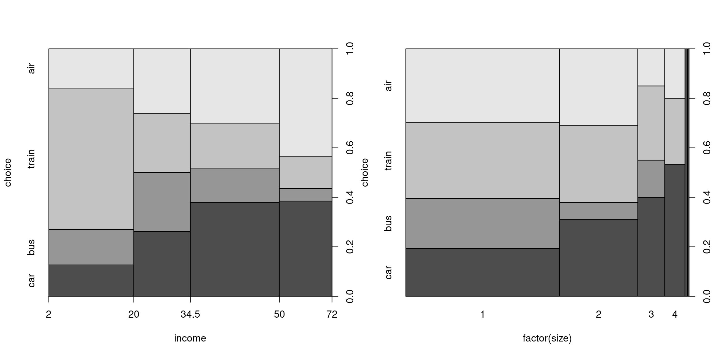

Figure 5.6: Marginal Influence of Individual-Specific Variables

Conditional influence of alternative-specific variables based on long format, e.g.:

plot(choice ~ travel, data = tm_long, breaks = 5,
  subset = mode == "air",  main = "air")

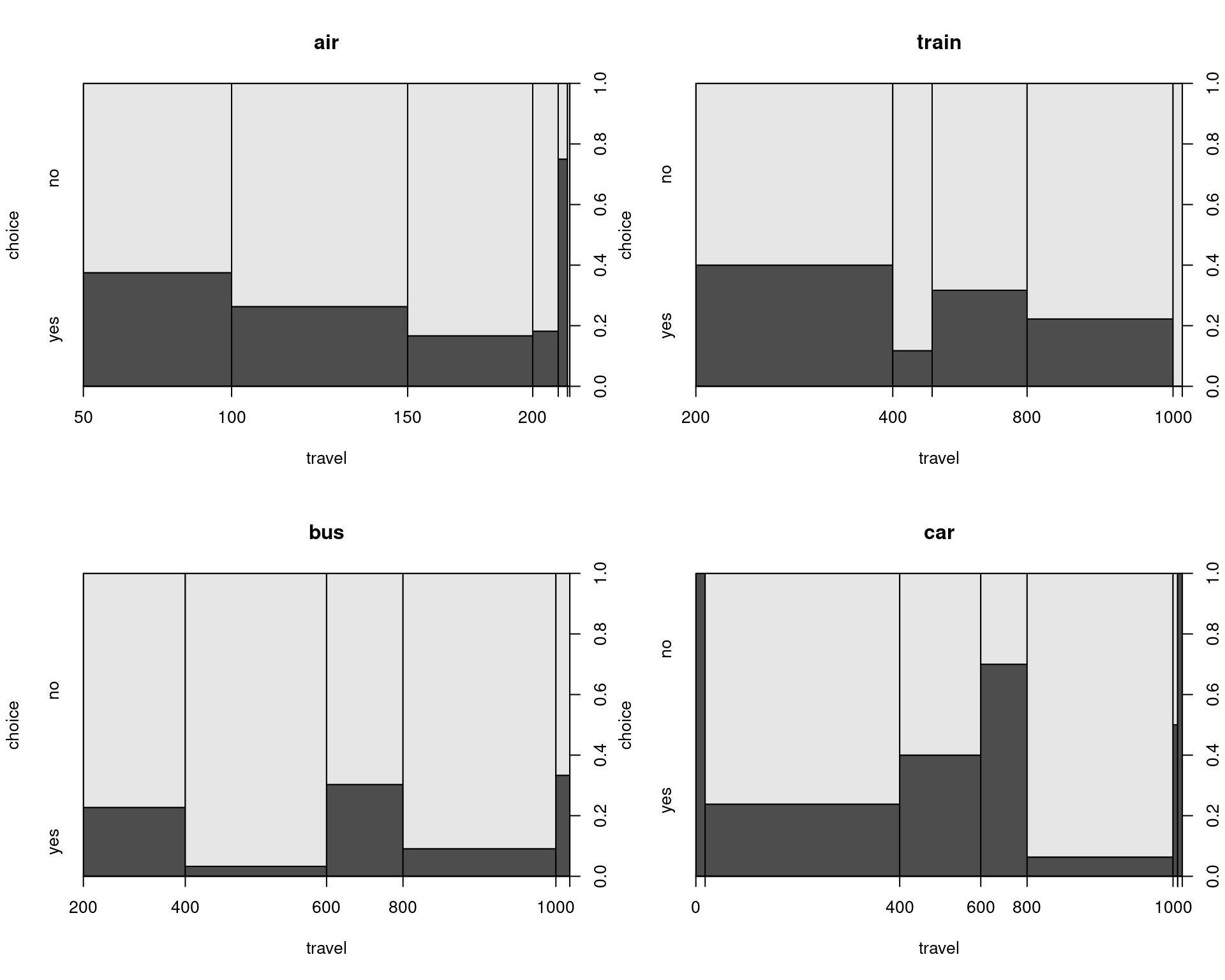
Figure 5.7: Conditional Influence of Alternative-Specific Variables

Or using lattice displays: Boxplots instead of spinograms.

library("lattice")
print(bwplot(choice ~ travel | mode, data = tm_long))

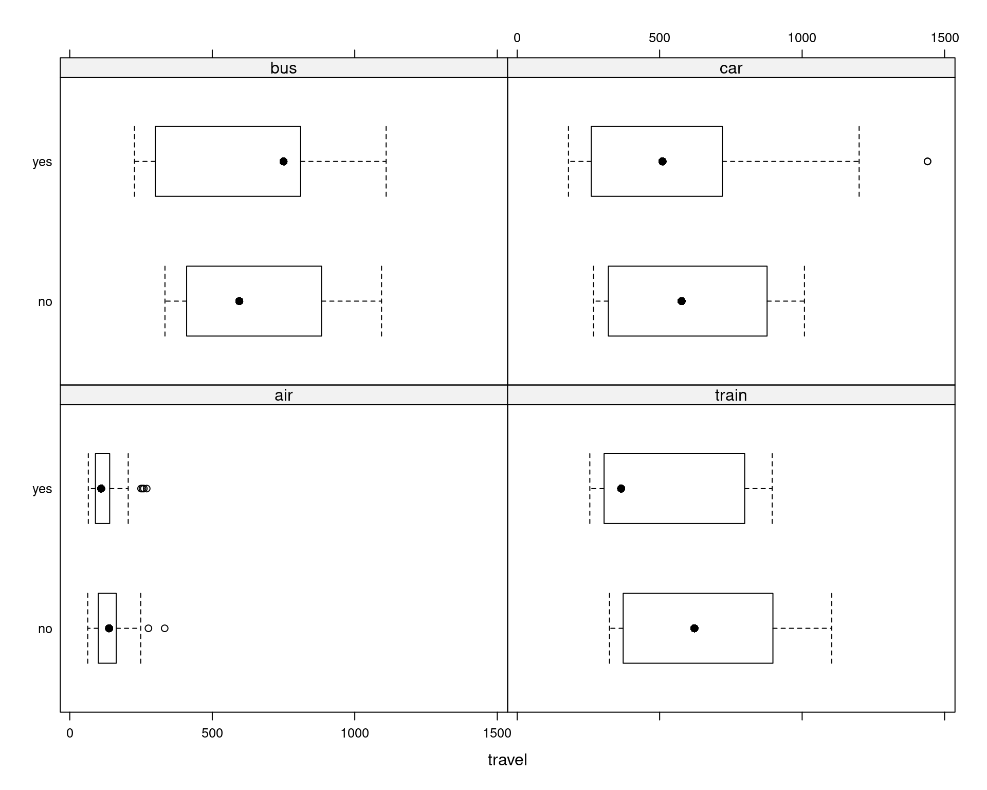
Figure 5.8: Influence Visualized in Boxplots

Relationship between alternative-specific variables:

print(xyplot(travel ~ wait | mode, data = tm_long))

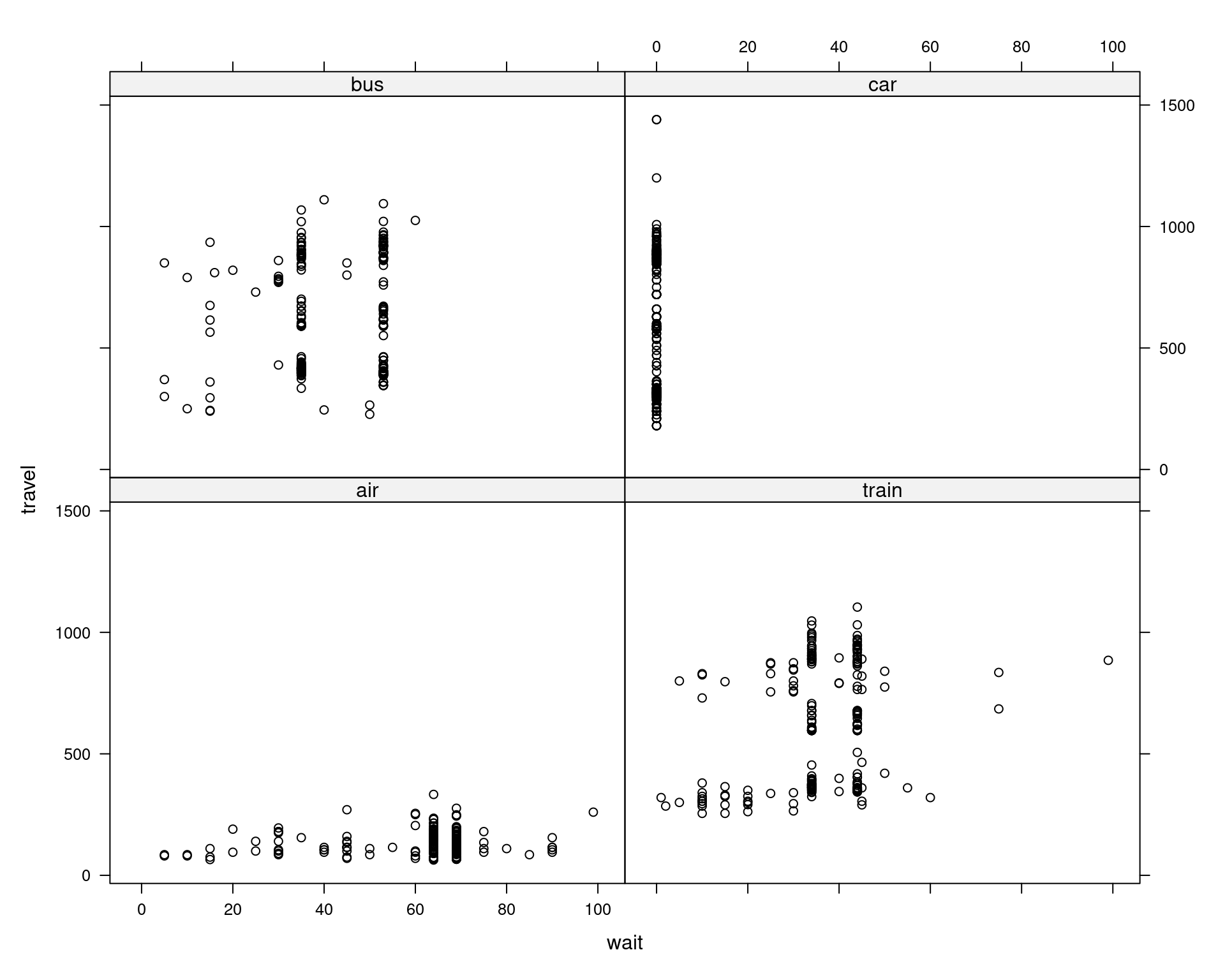
Figure 5.9: Relationship between Travel Time and Waiting Time

Modeling in R: The function mlogit() can estimate all three types of models:

• Conditional logit: y ~ z | 1 (or y ~ z for short).
• Multinomial logit: y ~ 0 | x.
• Mixed/hybrid logit: y ~ z | x.

The data can be prepared either on the fly (see above) or in advance using mlogit.data().

From long format:

tm <- mlogit.data(tm_long, shape = "long",
  choice = "choice", alt.var = "mode")

From wide format:

tm2 <- mlogit.data(tm_wide, shape = "wide",
  choice = "choice", varying = 4:19)

As an example, see a conditional logit model for travel mode choice using generalized cost, waiting time, and income-air interaction (Greene 2003, Table 21.11). This way, the individual-specific income variable is only used for choice of airplane.

tm$incair <- with(tm, income * (mode == "air"))
tm_cl <- mlogit(choice ~ gcost + wait + incair,
  data = tm, reflevel = "car")
modelsummary(list("Conditional logit"=tm_cl), 
             fmt=3, estimate="{estimate}{stars}")

	Conditional logit
(Intercept) × air	5.207***
	(0.779)
(Intercept) × train	3.869***
	(0.443)
(Intercept) × bus	3.163***
	(0.450)
gcost	-0.016***
	(0.004)
wait	-0.096***
	(0.010)
incair	0.013
	(0.010)
Num.Obs.	840
AIC	410.3
RMSE	0.59
mcfadden's r2	0.2982476988693

An extension of Greene’s model is the following mixed/hybrid logit model for travel mode choice using alternative-specific variables travel time and waiting time, and individual-specific variables income and party size.

tm_ml <- mlogit(choice ~ travel + wait | income + size,
  data = tm, reflevel = "car")
modelsummary(list("Mixed logit"=tm_ml, "Conditional logit"=tm_cl), 
             fmt=3, estimate="{estimate}{stars}")

	Mixed logit	Conditional logit
(Intercept) × air	5.538***	5.207***
	(1.042)	(0.779)
(Intercept) × train	5.523***	3.869***
	(0.705)	(0.443)
(Intercept) × bus	4.497***	3.163***
	(0.792)	(0.450)
travel	-0.004***
	(0.001)
wait	-0.101***	-0.096***
	(0.011)	(0.010)
income × air	0.008
	(0.013)
income × train	-0.063***
	(0.015)
income × bus	-0.021
	(0.016)
size × air	-0.929***
	(0.263)
size × train	0.172
	(0.230)
size × bus	-0.199
	(0.338)
gcost		-0.016***
		(0.004)
incair		0.013
		(0.010)
Num.Obs.	840	840
AIC	368.2	410.3
RMSE	0.66	0.59
mcfadden's r2	0.390057190340267	0.2982476988693

5.5 Independence of Irrelevant Alternatives

In MNL and CL models, we have a linear predictor of either of the below forms, or a combination of the two:

\[\begin{eqnarray*} \log\left( \frac{\pi_{ij}}{\pi_{is}} \right) & = & x_i^\top (\beta_j - \beta_s), \quad \mbox{or}\\ \log\left( \frac{\pi_{ij}}{\pi_{is}} \right) & = & (z_{ij} - z_{is})^\top \gamma. \end{eqnarray*}\]

For the individual-specific variables, it is the difference in coefficients, while for alternative-specific variables, it is the difference in attributes that is relevant and is driving the log-odds of a certain response category against the base category. A potential problem with this specification is that no other alternatives are influenced by this. In other words, the odds between two alternatives \(j\) and \(s\) only depend on the corresponding two probabilities (but not those of other alternatives). However, when there are alternatives that are similar to, or correlated with a certain alternative that is modeled, we would expect that not only the odds of these two categories are involved, but also those of other alternatives. This is known as independence of irrelevant alternatives (IIA). IIA is a realistic assumption if all alternatives can be clearly distinguished (e.g., certain brands). However, it is unrealistic if some alternatives are very similar (e.g., new bus/train line).

As a simple example, let’s say we have a hypothetical model of travel mode choice with two alternatives: “car” or “blue bus”, where person \(i\) is indifferent between these two alternatives: \(\pi_c = \pi_{bb} = 0.5\) and thus the corresponding odds are \(\pi_c / \pi_{bb} = 1\). If a new bus line, say “red bus” is introduced, and person \(i\) is indifferent between taking the blue or the red bus, thus \(\pi_{rb} / \pi_{bb} = 1\), independence of irrelevant alternatives would imply \(\pi_c / \pi_{bb} = 1\) remains unchanged. This can only be accomplished for \(\pi_c = \pi_{bb} = \pi_{rb} = 1/3\), i.e., if person \(i\) is indifferent between all of the alternatives. However, we would expect that the probability of taking the car, \(\pi_c = 0.5\) remains unchanged and thus \(\pi_{rb} = \pi_{bb} = 0.25\). Thus, MNL would underestimate \(\pi_c\) in this situation. This comes from the way the error terms were integrated out in the random utility model, where we assumed these error terms to be independent. It is possible to estimate the model without the assumption of independent error terms, but it complicates the model substantially. In practice, thus, two alternatives should not be too similar or too correlated in the model.

Advantages of IIA models:

• Parameters can be estimated consistently for subsets alternatives.
• Relevant if \(m\) is very large: Can save computation time and data collection, e.g.: If only bus vs. car is of interest, do not collect data for other means of transportation.

The classical test for the independence of irrelevant alternatives hypothesis proceeds by omitting one (or more) of the alternatives and then re-estimating the model, as parameters that do not pertain to a given category should not influence the other parameters. Thus, parameters \(\hat \gamma\) (and/or \(\hat \beta\)) need to be estimated once for the full set of alternatives and then for a subset of alternatives. Under IIA, both estimates should be similar. The estimates can be compared in a so-called Hausman-type specification test, which uses a quadratic form in the difference between parameters, scaled by the inverse of the difference of the estimated covariance matrices:

\[\begin{equation*} H ~=~ (\hat \gamma_\mathit{full} ~-~ \hat \gamma_\mathit{sub})^\top \left\{ \widehat{Var}(\hat \gamma_\mathit{full}) ~-~ \widehat{Var}(\hat \gamma_\mathit{sub}) \right\}^{-1} (\hat \gamma_\mathit{full} ~-~ \hat \gamma_\mathit{sub}) \end{equation*}\]

The general concept of the test is not confined to multinomial logit models; Hausman-type tests can be found in different econometric setups. This particular specification of the test, used for testing independence or irrelevant alternatives, is called the Hausman-McFadden test.

The main problem with the application of the test is that it is typically not clear which subset should be tested. In practice, usually several tests are carried out, sometimes one for each subset. Further care is required because of potential identification problems of some parameters.

As an example in R, we are going to drop the air alternative from the Australian travel data, since it is the alternative that stands out the most among the four.

tm_cl1 <- mlogit(choice ~ gcost + wait, data = tm,
  reflevel = "car")
tm_cl2 <- update(tm_cl1, alt.subset = c("train", "bus", "car"))
hmftest(tm_cl1, tm_cl2)

## 
##  Hausman-McFadden test
## 
## data:  tm
## chisq = 33, df = 4, p-value = 1e-06
## alternative hypothesis: IIA is rejected

First, the mlogit function is called and the reference level is set to car. Then, the model is refitted in a convenient way, without repeating the entire function call, using the update function, specifying the vector of alternatives we want to fit with the alt.subset argument. Having set up the two models, we can use the hmftest() function to test for independence or irrelevant alternatives. Given the p-value, we reject the null hypothesis and conclude that we do not have IIA in this model.

5.6 Generalized Multinomial Response Models

The source of IIA in the multinomial logit models we have seen so far is the assumption of independence of the error terms \(\varepsilon_{ij}\) in the random utility model formulation \(u_{ij} = \eta_{ij} + \varepsilon_{ij}\). Independent errors in RUMs imply that the utility of one alternative being higher or lower than average for person \(i\) is not correlated with the utility of another alternative being higher or lower than average. In many applications, though, errors are likely not to be independent.

There are different conceivable extensions to relax the assumption of independent error terms, including:

• Multinomial probit (MNP) models, where error terms have multivariate normal distribution \((\varepsilon_{i1}, \dots \varepsilon_{im})^\top \sim \mathcal{N}(0, \Sigma)\) with non-spherical errors \(\Sigma \neq \sigma^2 \cdot I\). In words, we assume that the error term for person \(i\) and the \(m\) alternatives have some sort of correlation structure. This approach thus requires estimation of the full variance-covariance matrix \(\Sigma\). Since the number of variances and covariances increases quadratically in the number of alternatives \(m\), solving the integral in the random utility model becomes more and more complicated as the number of alternatives grows. Specifying the model thus becomes more challenging, and so does optimizing the likelihood (often done by using Markov chain Monte Carlo techniques in a Bayesian setting).
• Mixed effects logit (MXL) models, where additional dependence is generated via random effect terms. These added random effects can be individual- or alternative-specific, and are zero on average, but might deviate from zero for a given individual.
• Nested logit models, where dependence is generated by nesting alternatives in tree structure, i.e., we assume that the decision is not made at once between the \(m\) alternatives, but in a recursive way. For example, having four alternatives, one might first make a decision between 2-2 alternatives, and then choose an alternative from the remaining two at the next nesting level.

5.6.1 Travel mode choice: Nested logit

To illustrate this nested structure, we set up a nested logit model for travel mode choice, where persons first choose whether to fly ("air") or to use ground transportation ("car", "train", "bus"), and, if ground transportation is chosen, the decision between the three remaining alternatives is made consequently, at the second nesting level. This way of setting up the model reflects that the choice of flying vs. ground travel and the choice among the three ground transportation modes, respectively, is driven by two different sets of variables.

Two equivalent formulations of the likelihood function are:

\[\begin{eqnarray*} L_i & = & \pi_{i1}^{d_{i1}} ~ \pi_{i2}^{d_{i2}} ~ \pi_{i3}^{d_{i3}} ~ \pi_{i4}^{d_{i4}}\\ & = & \pi_{i1}^{d_{i1}} ~ \pi_{ig}^{d_{i2} + d_{i3} + d_{i4}} ~\cdot~ \left( \frac{\pi_{i2}}{\pi_{ig}} \right)^{d_{i2}} \left( \frac{\pi_{i3}}{\pi_{ig}} \right)^{d_{i3}} \left( \frac{\pi_{i4}}{\pi_{ig}} \right)^{d_{i4}}, \end{eqnarray*}\]

The first way of formulating the likelihood reflects the probability that person \(i\) chooses, let’s say, alternative \(1\), to the power of \(d_{i1}\), where \(d_{i1}\) is an indicator of whether the alternative was chosen or not. The dummy variable pertaining to the chosen alternative takes up \(1\) as a value, while the rest of the dummy variables are necessarily zero and thus only the probability that person \(i\) chooses the given alternative remains, as all other terms cancel out.

In the second line we have a completely equivalent way of formulating the problem, where a decision is first made between flying and ground travel (binomial decision), which means either \(d_{i1}=1\), if air travel is chosen, or the sum of the remaining three dummy variables \(d_{i2}+d_{i3}+d_{i4}=1\), if ground travel is chosen. Then, in a second part, we formulate a multinomial model for choosing among the three means of ground travel, with their corresponding probabilities scaled by the probability of choosing ground travel \(\pi_{ig} = \pi_{i2} + \pi_{i3} + \pi_{i4}\). This way of rewriting the likelihood becomes important in particular if covariance is assumed to play a role: it makes a difference whether the covariance is linked to the three scaled variables, or the raw probabilities in the original formulation. In terms of fitting the model, an advantage of this formulation is that the model stays multiplicative in likelihood, thus log-likelihood is additive, and we get two separate sums: one for ground travel choice, and one for air travel vs. ground travel, which means the two models can be fitted separately.

To illustrate this example in R, we first fit a binary GLM, where the dependent variable I(choice == "air") is a (binary) logical variable, which is TRUE for air travel and FALSE for any of the three ground travel modes. In this binary GLM, we assume that some individual-specific variables have an effect, namely income and travel party size, as we have found these to be particularly important in the decision of whether or not to choose air travel. (Note that instead of creating the dependent variable on the fly, we could also add it to the data set before fitting the model.) Then, we fit a multinomial logit model for ground travel choice (alt.subset = c("train", "bus", "car")), explained by generalized cost and waiting time, both alternative-specific variables.

tm_fly <- glm(I(choice == "air") ~ income + size,
  data = tm_wide, family = binomial)
tm_ground <- mlogit(choice ~ gcost + wait, data = tm,
  reflevel = "car", alt.subset = c("train", "bus", "car"))
modelsummary(list("Air travel binomial"=tm_fly, 
                  "Ground travel multinomial logit"=tm_ground), 
             fmt=3, estimate="{estimate}{stars}")

	Air travel binomial	Ground travel multinomial logit
(Intercept)	-1.417***
	(0.421)
income	0.030***
	(0.008)
size	-0.384*
	(0.181)
(Intercept) × train		4.464***
		(0.641)
(Intercept) × bus		3.105***
		(0.609)
gcost		-0.064***
		(0.010)
wait		-0.070***
		(0.015)
Num.Obs.	210	456
AIC		183.9
BIC
Log.Lik.
F	7.180
RMSE	0.43	0.73
mcfadden's r2		0.450392412997331

We can see from the alternative-specific intercepts in the multinomial logit model that if all explanatory variables are zero, there would be a strong preference for train and bus over car. However, this is unlikely to happen: costs are never zero, and neither is the waiting time for train and bus, whereas for car it is always zero. Thus, the intercepts reflect a situation that does not occur in practice. With increasing cost and waiting time, it becomes less and less likely to choose the alternative for which cost and/or waiting time has increased, and more likely to choose any of the other alternatives.

5.6.2 Malformations of the CNS

In this section, we are taking an example from biostatistics, where using a nested logit model works well and is intuitive. The goal is to examine whether there is a link between water hardness and malformations of the central nervous system. In case poor quality tap water might increase the risk of certain diseases, including malformations of the CNS, authorities should try to improve tap water quality in the given area, and therefore it is important to investigate this issue. We look at two specific malformations: Anencephalus and Spina Bifida, and have a third option for other types of CNS malformations.

Though the data frame we are using has only 16 observations, the underlying data set is indeed large: it contains aggregated data on the number of live births from different areas of South Wales, UK, where for each area we have counts for the number of births with no malformation, and with any of the three types of malformations.

The data frame containing 16 observations on 7 variables:

Table 5.4: Variables in the CNS Malformations Data Set

Variable	Description
Area	Area in South Wales.
NoCNS	Count of births with no CNS malformation.
An	Count of Anencephalus births.
Sp	Count of Spina Bifida births.
Other	Count of other births with CNS malformation.
Water	Water hardness.
Work	Type of work (manual, non-manual) done by parents.

We first load the data:

data("cns", package = "faraway")

Next, using the reshape function, the data is transformed from wide format to long format for further explanatory analysis. For visualization with a mosaic plot, the water variable is cut into four (relatively arbitrary) categories. First, we create a contingency table (cns_tab) of the number of cases explained by the discretized water quality variable, by the CNS malformation type, and the work variable.

cns2 <- reshape(cns, direction = "long",
  timevar = "cns", times = names(cns)[2:5],
  varying = 2:5, v.names = "cases")[, 2:5]
cns2$Water2 <- with(cns2, cut(Water, fivenum(Water),
  include.lowest = TRUE))
cns_tab <- xtabs(cases ~ Water2 + cns + Work, data = cns2)

Then, we can use the spineplot() function on our multi-way contingency table to create two separate mosaic plots - one for manual work and one for non-manual work. (Note that mosaicplot() is more difficult to use here because it has not control of ylim. Since overall probabilities are small, we plot them only up until 1.2%.)

spineplot(cns_tab[, c(2, 3, 4, 1), 1], ylim = c(0, 0.012),
  tol = 0, off = 0, main = "Work = Manual")
spineplot(cns_tab[, c(2, 3, 4, 1), 2], ylim = c(0, 0.012),
  tol = 0, off = 0, main = "Work = NonManual")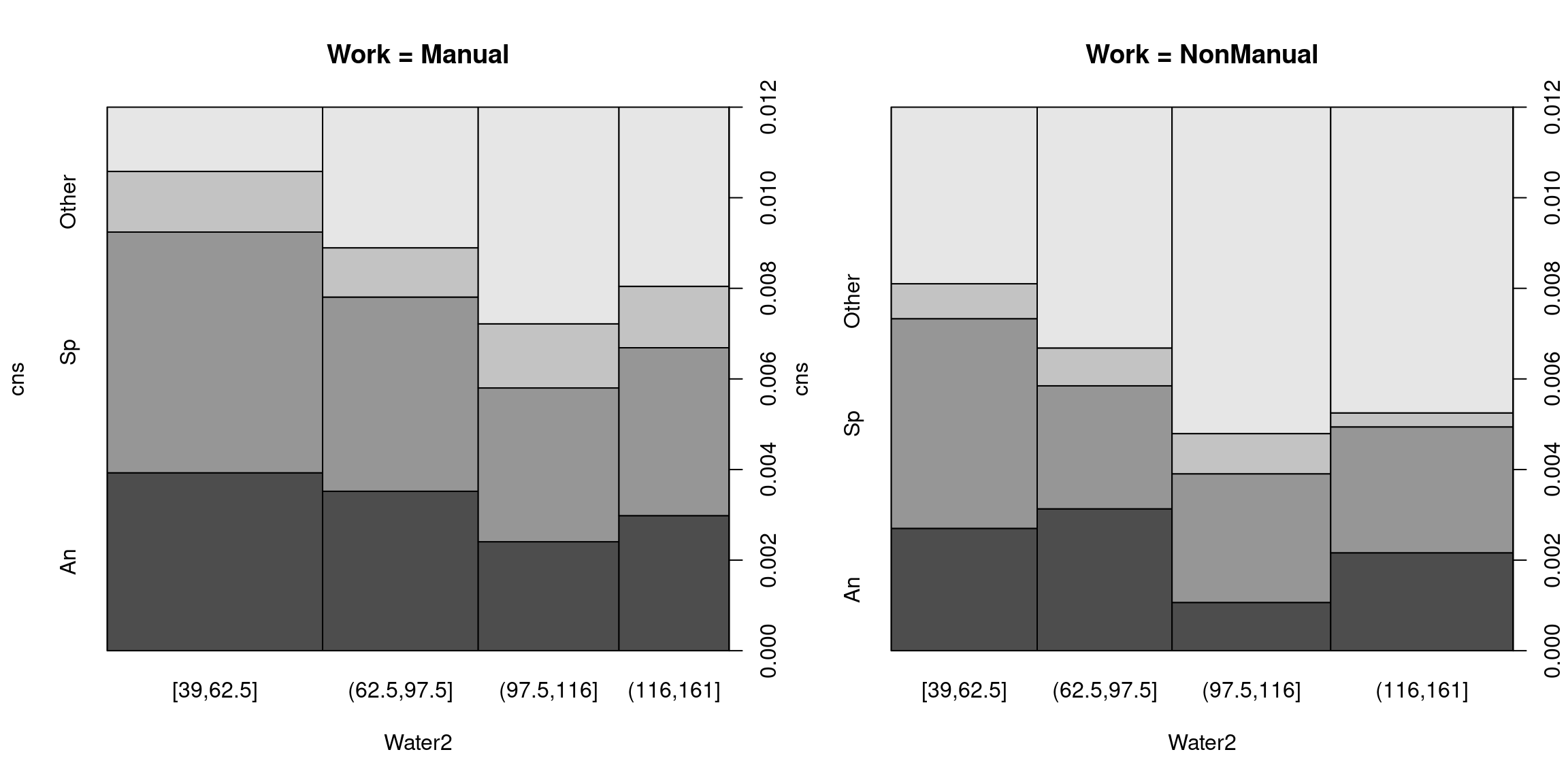

Figure 5.10: Spineplot Visualization of CNS Malformations for Manual and Non-Manual Work

We can see that there is a similar pattern for manual and non-manual work, although the overall level is a bit lower for non-manual work. With increasing water hardness, the probability of malformations seems to be decreasing. If we look at the non-manual work group, the probability goes down from around 1% to 0.7%. Although this may sound like a small change, it has enormous implications for the occurrence of these rare diseases. We can furthermore see from the mosaic plots that there might be an optimal point - too hard water might have a negative effect again - but for now, we look at a linear specification to test whether the probability of CNS malformations decrease with increasing water hardness.

To model whether risk factors Water and Work drive the occurrence of CNS malformations, the wide version of the data set is used. Using the glm() function, we set up a nested logit model, where in the first nesting step we ask whether there is any malformation, and in the second nesting step we look at the type of malformation. This is a natural setup as the two options: malformation/no malformation are clearly separable, whereas the type of malformation might not be that easy to separate since they are related diseases. Thus, nesting in this case is rather intuitive.

The glm() function can be used for a matrix response with two columns: in the first column, the number of successes, and in the second column, the number of failures. In this data set, successes are the occurrence of any type of malformation, since this is the probability we want to model. We explain these variables by water and work.

cns$CNS <- cns$An + cns$Sp + cns$Other
cns_logit <- glm(cbind(CNS, NoCNS) ~ Water + Work,
  data = cns, family = binomial)
modelsummary(list("CNS binomial logit"=cns_logit), 
             fmt=3, estimate="{estimate}{stars}")

	CNS binomial logit
(Intercept)	-4.433***
	(0.090)
Water	-0.003***
	(0.001)
WorkNonManual	-0.339***
	(0.097)
Num.Obs.	16
AIC	102.5
BIC	104.8
Log.Lik.	-48.245
F	13.593
RMSE	0.00

Looking at the resulting coefficient test, both variables are highly significant: parents doing non-manual work are considerably less likely to suffer a birth with a CNS malformation. \(exp(-0.33)=0.71\), which means there is an almost 30% reduction in the occurrence of CNS malformations for non-manual work compared to manual work, given the same level of water hardness. Furthermore, if water hardness increases by one unit, the odds of a CNS malformation occurring decrease by 0.3%. Scaling this, we can say that increasing water hardness by 10 units decreases the odds of a CNS malformation by around 3%. The corresponding effect plots are:

plot(allEffects(cns_logit), rescale.axis = FALSE)

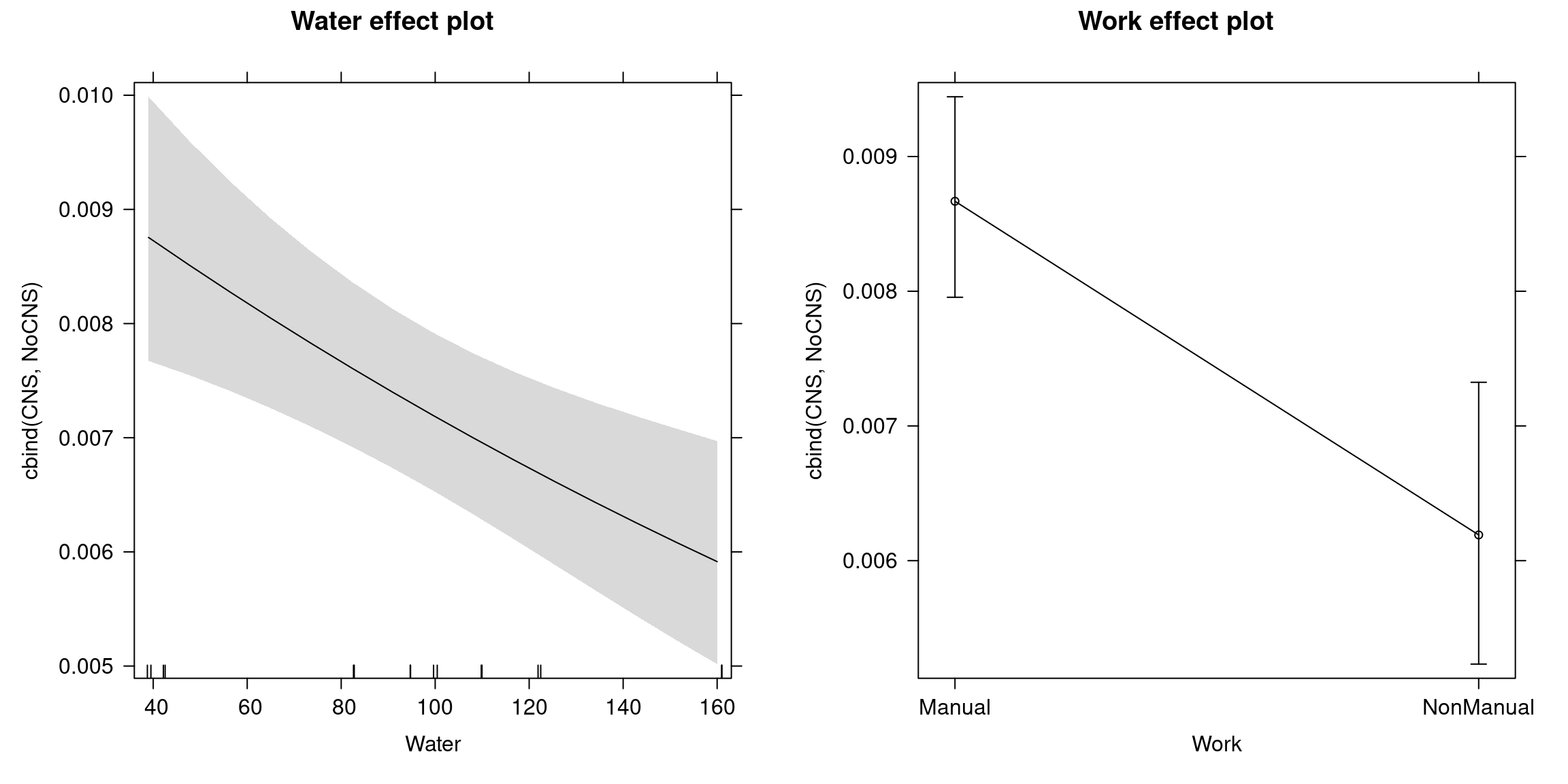
Figure 5.11: Water Hardness and Work Effects on CNS Malformations

Then, in a second step, we model whether the type of malformation also depends on these variables. For this, we use the multinom() function for the three types of malformations. First, we fit a model with two explanatory variables: water and work. Second, another model with only alternative-specific intercepts is fitted.

cns_mnl <- multinom(cbind(An, Sp, Other) ~ Water + Work,
  data = cns, trace = FALSE)
cns_mnl1 <- multinom(cbind(An, Sp, Other) ~ 1,
  data = cns, trace = FALSE)
modelsummary(list("CNS multinomial logit"=cns_mnl, 
                  "Intercept-only"=cns_mnl1), 
             fmt=3, estimate = "{estimate} {stars}", shape = response + term ~ model)

response		CNS multinomial logit	Intercept-only
Sp	(Intercept)	0.375 *	0.290 ***
		(0.190)	(0.083)
	Water	-0.001
		(0.002)
	WorkNonManual	0.116
		(0.209)
Other	(Intercept)	-1.123 ***	-0.981 ***
		(0.280)	(0.120)
	Water	0.002
		(0.003)
	WorkNonManual	-0.270
		(0.325)
	Num.Obs.	16	16
	R2	0.002	0.000
	R2 Adj.	0.001	-0.001
	AIC	1383.5	1378.5
	BIC	1388.2	1380.0
	RMSE	0.11	0.11

lrtest(cns_mnl, cns_mnl1)

## Likelihood ratio test
## 
## Model 1: cbind(An, Sp, Other) ~ Water + Work
## Model 2: cbind(An, Sp, Other) ~ 1
##   #Df LogLik Df Chisq Pr(>Chisq)
## 1   6   -686                    
## 2   2   -687 -4  2.93       0.57

Comparing the two models with a likelihood ratio test, we get a p-value of 57%, and thus we can say that based on the data, we cannot conclude anything about the type of malformation occurring - water hardness and work type do not seem to have a significant effect on the type of malformation.

The intercept-only model above reflects the conditional occurrence probabilities (given any type of CNS malformation).

head(fitted(cns_mnl1), 1)

##       An     Sp  Other
## 1 0.3689 0.4928 0.1383

Thus, our findings in short are: Doing manual work and drinking too soft water increase the risk of CNS malformations occurring in general. However these variables do not significantly influence which malformation occurs.

5.6.3 Further models

Multinomial models in economics and business applications are particularly popular in the area of marketing (brand choice models) and transport economics (travel mode choice models), among others.

With Bayesian modeling of multinomial probit models, it is possible to incorporate correlation structures of error terms directly into the random utility model. These models are typically estimated by simulation-based techniques, e.g., Markov chain Monte Carlo. For consistent estimation it is typically required, along with a large enough sample size (\(n \rightarrow \infty\)), to have a large enough number of simulations \(s \rightarrow \infty\), to get valid inference

Other R packages:

• MNP: Multinomial probit models.
• bayesm: Bayesian inference for marketing and microeconometrics.