Chapter 8 Limited Dependent Variables
8.1 Introduction
Limited response variables: Mixed discrete and continuous features of the dependent variable.
Typical sources: Censoring and truncation.
Economic explanations:
- Corner solutions: Utility-maximizing choice of individuals is at the corner of the budget set, typically zero.
- Sample selection: Data deficiency causes response to be unknown (or different) for subsample.
- Treatment effects: Response for each individual is only observable for one level of a “treatment” variable.
Examples: Typical economic examples for limited responses.
- Labor supply.
\(y_i\): Number of hours worked by person \(i\).
Potential covariates: Education, non-work income, … - Expenditures for health services.
\(y_i\): Expenditures of person \(i\) for health services last month.
Potential covariates: Health status, income, gender, … - Wage equations.
\(y_i\): Earnings of person \(i\) derived from tax returns.
Potential covariates: Education, previous experience, … - Unemployment programs.
\(y_i\): Wage of person \(i\) after unemployment.
Treatment: Training program (potentially non-random assignment).
Potential covariates: Occupation, duration of unemployment, …
8.1.1 Example: PSID 1976 (Mroz data)
Cross-section data from the 1976 Panel Study of Income Dynamics (PSID), based on data for the previous year, 1975.
A data frame containing 753 observations on 21 variables, including:
| Variable | Description |
|---|---|
participation |
Did the individual participate in the labor force in 1975? (equivalent to wage \(> 0\) or hours \(> 0\)) |
hours |
Wife’s hours of work in 1975. |
youngkids |
Number of children less than 6 years old. |
oldkids |
Number of children between ages 6 and 18. |
age |
Wife’s age in years. |
education |
Wife’s education in years. |
wage |
Wife’s average hourly wage in 1975 (USD). |
fincome |
Family income in 1975 (USD). |
Example: Corner solution
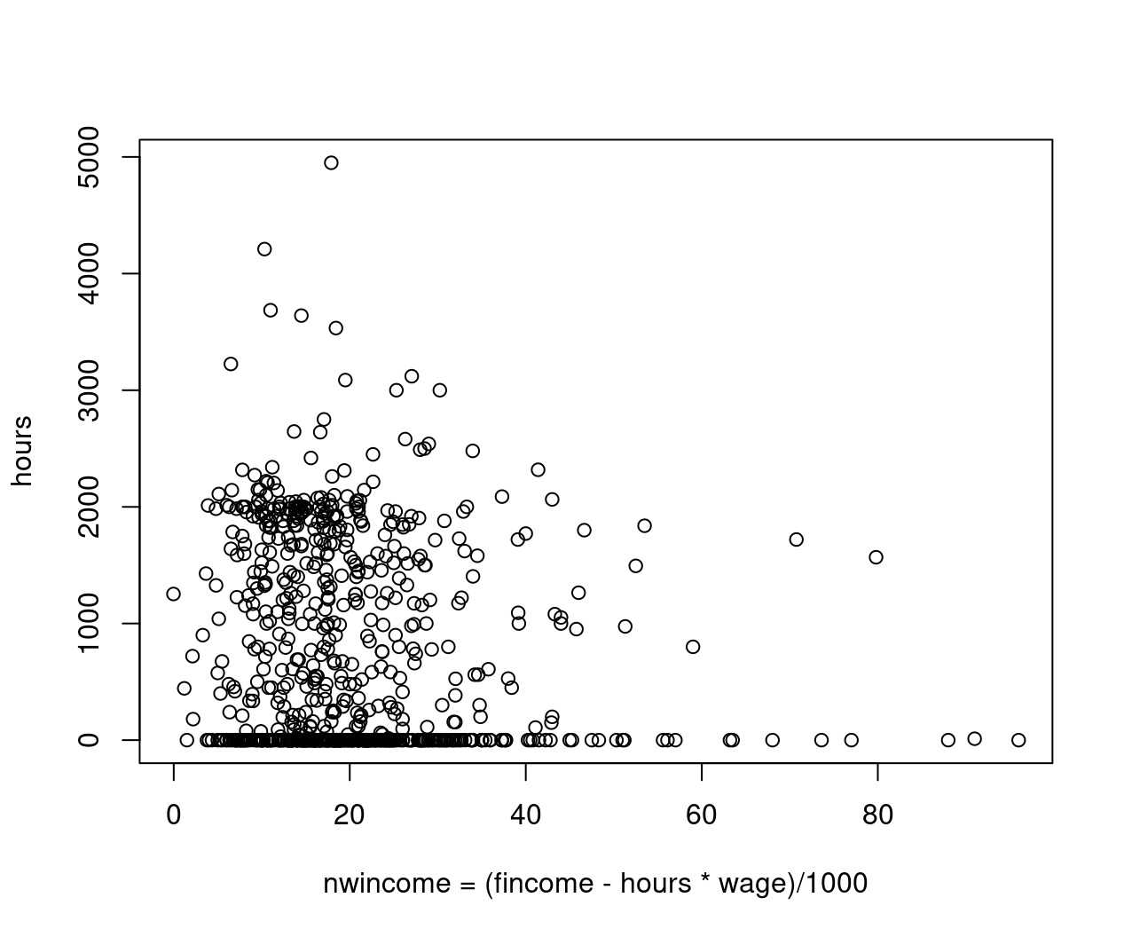
Figure 8.1: Nonwife income against hours worked - jittered
Example: Sample selection
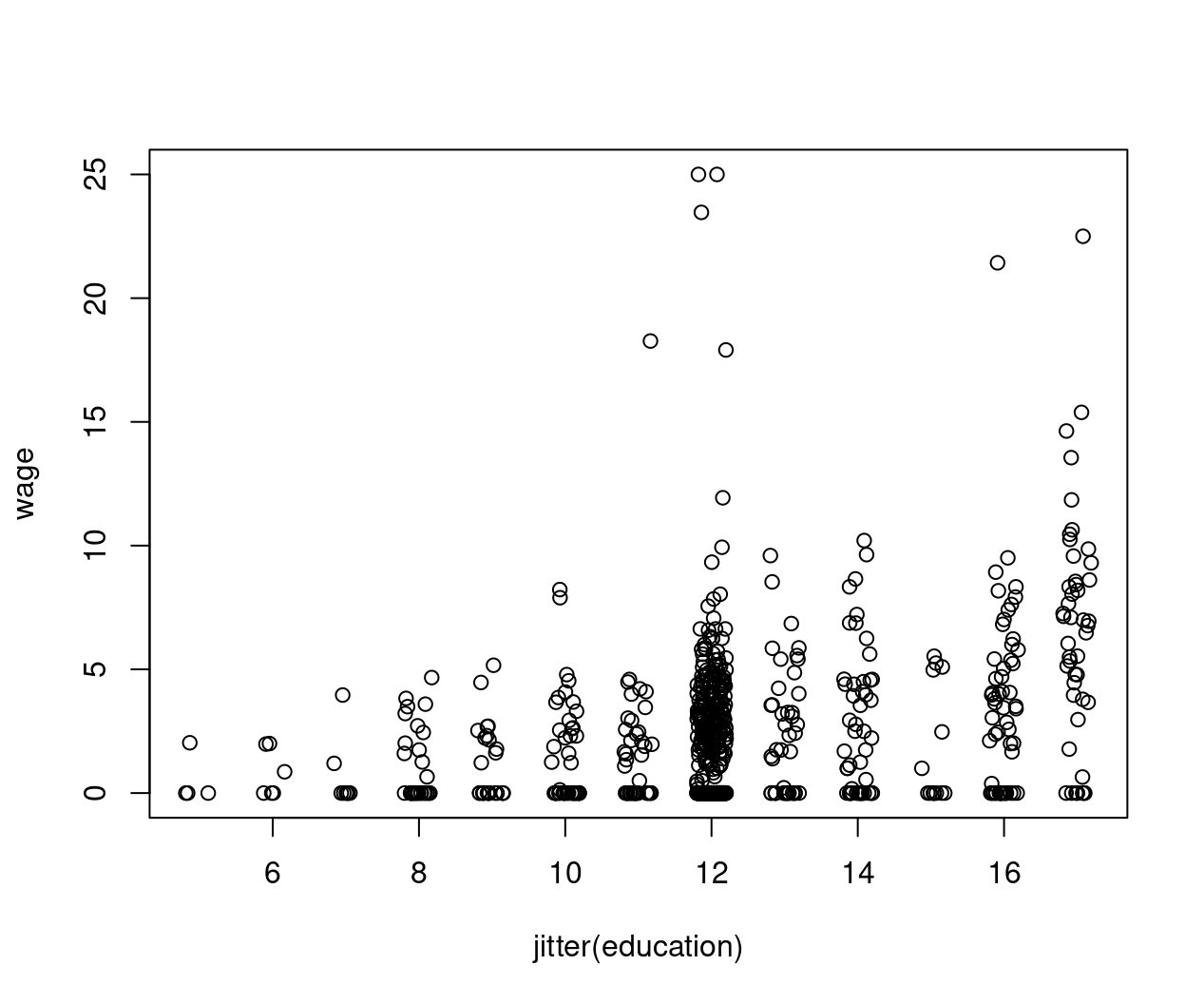
Figure 8.2: Education against wage - jittered
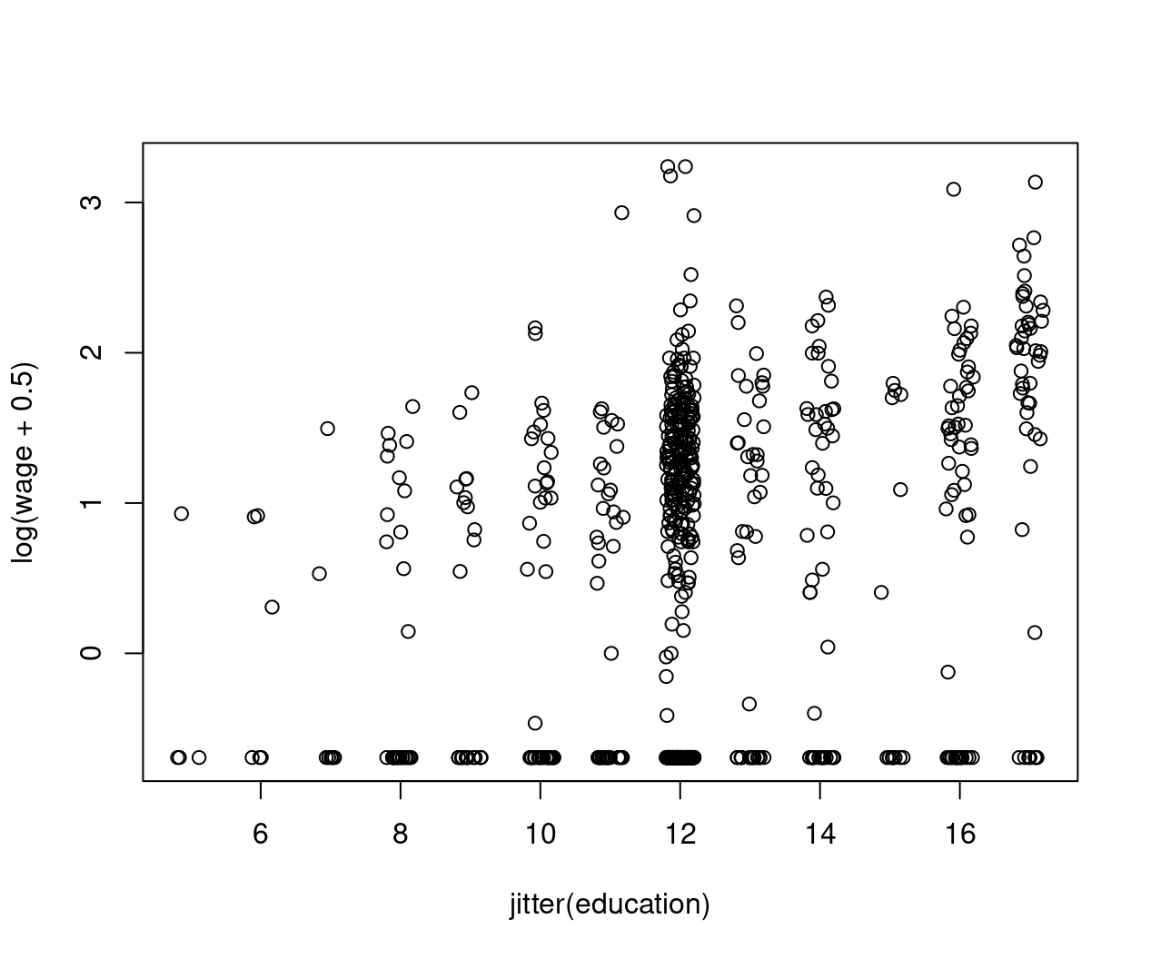
Figure 8.3: Education against log(wage+0.5) - jittered
8.2 Tobin’s Corner Solution Model
Problem: As motivated above, many microeconomic variables have
- non-negative values,
- a cluster of observations at zero.
Note: OLS cannot be used sensibly due to
- possibly negative predictions,
- imposed constant marginal effects (which cannot be remedied by logs as \(\log(0)\) is not defined).
Quantities of interest:
- \(\text{P}(y = 0 ~|~ x) = 1 - \text{P}(y > 0 ~|~ x)\), probability of zero.
- \(\text{E}(y ~|~ y > 0,~ x)\) expectation conditional on positive \(y\).
- \(\text{E}(y ~|~ x) = P(y > 0 ~|~ x) \cdot \text{E}(y ~|~ y > 0,~ x)\) expectation.
Ideas:
- Two-part model with binary selection and truncated outcome.
- Latent variable driving both selection and outcome.
Tobin’s solution: Employ the latter approach with latent Gaussian variable \(y^*\) and observed discrete-continuous response \(y\):
\[\begin{eqnarray*} y^* & = & x^\top \beta ~+~ \varepsilon, \qquad \varepsilon ~|~ x \sim \mathcal{N}(0, \sigma^2),\\ y\phantom{^*} & = & \max(0, y^*), \end{eqnarray*}\]
i.e., \(y\) is a censored version of \(y^*\).
Likelihood:
\[\begin{equation*} L(\beta, \sigma; y, x) ~=~ \prod_{i = 1}^n f(y_i ~|~ x_i, \beta, \sigma)^{I(y_i > 0)} \cdot \text{P}(y_i = 0 ~|~ x_i)^{I(y_i = 0)} \end{equation*}\]
where
\[\begin{eqnarray*} \text{P}(y_i = 0 ~|~ x_i) & = & \text{P}(y_i^* \le 0 ~|~ x_i) \\ & = & \Phi \left(\frac{0 - x_i^\top \beta}{\sigma} \right) ~=~ 1 - \Phi \left(\frac{x_i^\top \beta}{\sigma} \right) \\ f(y_i ~|~ x_i, \beta, \sigma) & = & \frac{1}{\sigma} \cdot \phi \left( \frac{y_i - x_i^\top \beta}{\sigma} \right) \end{eqnarray*}\]
Remarks:
- Model is known as tobit model.
- Despite the name it does not belong to the same model class as the binary logit and probit models.
- Log-likelihood can be shown to be globally concave.
- MLE is well-behaved (asymptotically normal etc.).
In R: tobit() from package AER. Convenience interface to survreg() from package survival which provides much more general regression tools for censored responses.
Alternatively: crch(..., left = 0) from package crch for censored regression with conditional heteroscedasticity. Dedicated interface for tobit-type models with either censoring or truncation, different response distributions (beyond normal).
Example: Regression for annual hours of work in PSID 1976 data, using reduced-form specification. Wage is missing as a regressor (as unobserved for non-working subsample).
Model equation of interest:
Fitting tobit model and naive OLS models:
hours_tobit <- tobit(hours_f, data = PSID1976)
hours_ols1 <- lm(hours_f, data = PSID1976)
hours_ols2 <- lm(hours_f, data = PSID1976,
  subset = participation == "yes")
Compare coefficients:
modelsummary(list("Tobit" = hours_tobit,
                  "OLS (all)" = hours_ols1,
                  "OLS (positive)" = hours_ols2),
fmt=3, estimate="{estimate}{stars}")| Tobit | OLS (all) | OLS (positive) | |
|---|---|---|---|
| (Intercept) | 965.305* | 1330.482*** | 2056.643*** |
| (446.436) | (270.785) | (346.484) | |
| nwincome | -8.814* | -3.447 | 0.444 |
| (4.459) | (2.544) | (3.613) | |
| education | 80.646*** | 28.761* | -22.788 |
| (21.583) | (12.955) | (16.434) | |
| experience | 131.564*** | 65.673*** | 47.005** |
| (17.279) | (9.963) | (14.556) | |
| I(experience^2) | -1.864*** | -0.700* | -0.514 |
| (0.538) | (0.325) | (0.437) | |
| age | -54.405*** | -30.512*** | -19.664*** |
| (7.419) | (4.364) | (5.894) | |
| youngkids | -894.022*** | -442.090*** | -305.721** |
| (111.878) | (58.847) | (96.450) | |
| oldkids | -16.218 | -32.779 | -72.367* |
| (38.641) | (23.176) | (30.361) | |
| Num.Obs. | 753 | 753 | 428 |
| R2 | 0.266 | 0.140 | |
| R2 Adj. | 0.259 | 0.126 | |
| AIC | 7656.2 | 12117.1 | 6863.2 |
| BIC | 7697.8 | 12158.7 | 6899.7 |
| Log.Lik. | -6049.534 | -3422.581 | |
| F | 38.495 | 9.792 | |
| RMSE | 953.68 | 746.18 | 718.92 |
8.2.1 Truncated normal distribution
Question: How can these models be interpreted?
Needed: Better understanding of truncated (normal) distributions.
Probability density function: Random variable \(y\) with density function \(f(y)\), truncated from below at \(c\). General form and \(\mathcal{N}(\mu, \sigma^2)\) distribution.
\[\begin{eqnarray*} f(y ~|~ y > c) & = & \frac{f(y)}{\text{P}(y > c)} ~=~ \frac{f(y)}{1 - F(c)} \\ & = & \frac{1}{\sigma} \cdot \phi\left( \frac{y - \mu}{\sigma} \right) \left/ \left\{ 1 - \Phi \left(\frac{c - \mu}{\sigma} \right) \right\} \right. \end{eqnarray*}\]
Example: Standard normal distribution truncated at \(c = -1\) and \(c = 0\).
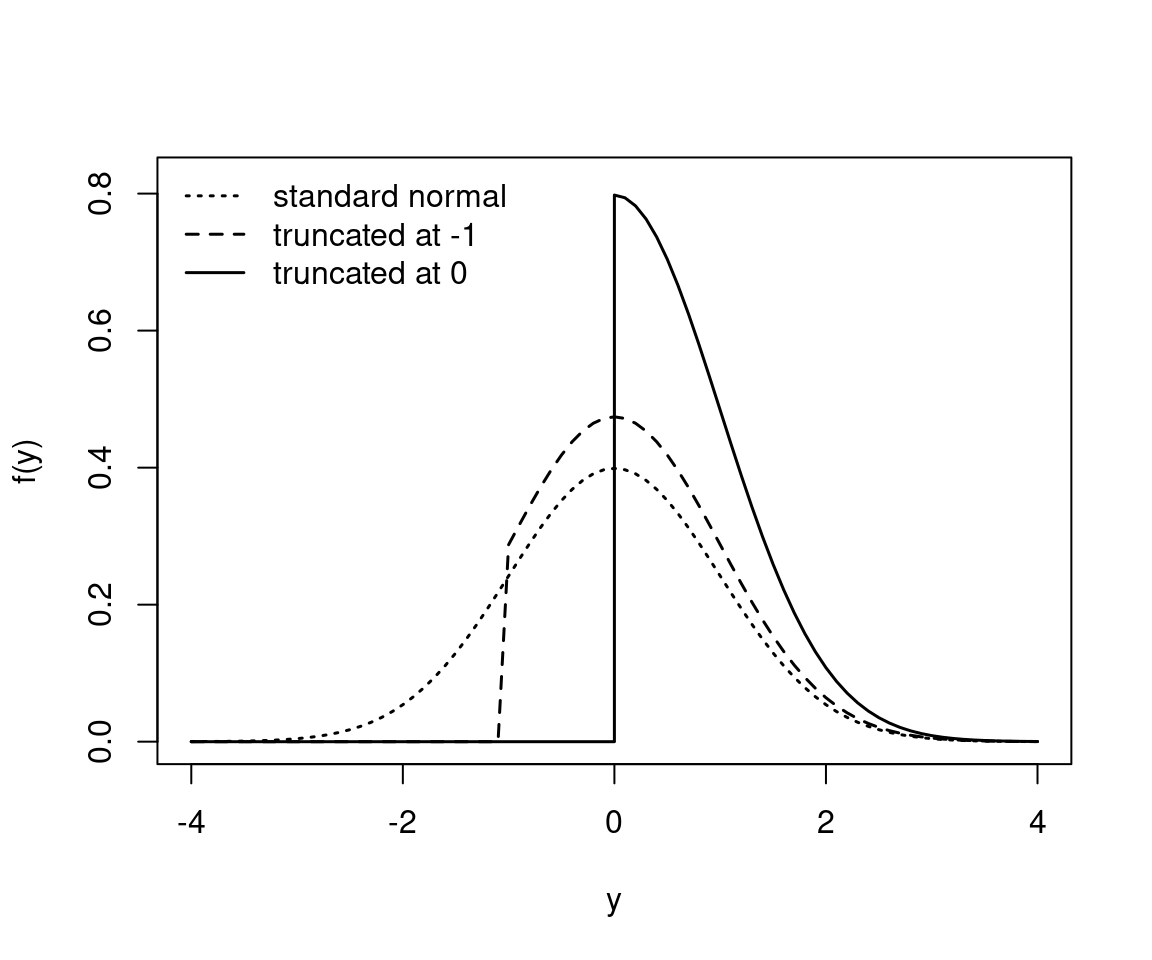
Figure 8.4: Standard normal distribution truncated at two different points
Expectation: For \(\varepsilon \sim \mathcal{N}(0, 1)\).
\[\begin{eqnarray*} \text{E}(\varepsilon ~|~ \varepsilon > c) & = & \int_c^\infty \varepsilon \cdot f(\varepsilon ~|~ \varepsilon > c) ~d \varepsilon \\ & = & \frac{1}{1 - \Phi(c)} ~ \int_c^\infty \varepsilon \cdot \phi(\varepsilon) ~d \varepsilon \\ & = & \frac{1}{1 - \Phi(c)} ~ \left\{ \left. - \phi(\varepsilon) \phantom{\frac{.}{.}} \! \right|_c^\infty \right\} \\ & = & \frac{\phi(c)}{1 - \Phi(c)} \end{eqnarray*}\]
Because \(\phi'(x) = -x \cdot \phi(x)\).
Note: This simple solution does not hold in general.
Inverse Mills ratio: Defined as
\[\begin{equation*} \lambda(x) ~=~ \frac{\phi(x)}{\Phi(x)}. \end{equation*}\]
Hence, due to symmetry of the normal distribution, the following holds for \(\varepsilon \sim \mathcal{N}(0, 1)\) and \(y \sim \mathcal{N}(\mu, \sigma^2)\), respectively:
\[\begin{eqnarray*} \text{E}(\varepsilon ~|~ \varepsilon > c) & = & \lambda(-c), \\ \text{E}(y ~|~ y > c) & = & \mu ~+~ \sigma \cdot \lambda\left(\frac{\mu - c}{\sigma}\right). \end{eqnarray*}\]
Example: \(y \sim \mathcal{N}(\mu, 1)\) with truncation at \(c = 0\).
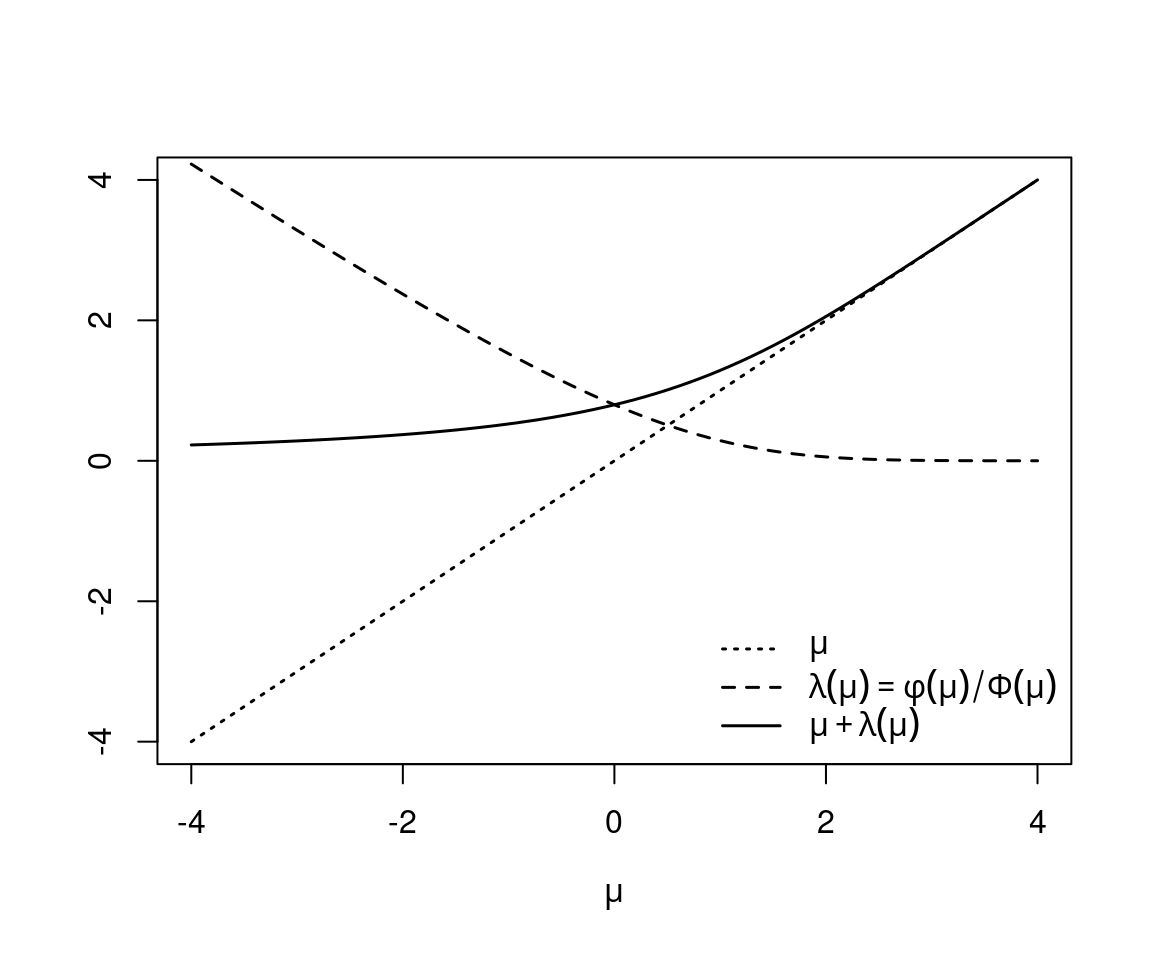
Figure 8.5: Mean and Inverse Mills ratio
8.2.2 Interpretation of the tobit model
Uninteresting: Expectation of latent variable is straightforward but lacks substantive interpretation.
\[\begin{equation*} \text{E}(y^* ~|~ x) ~=~ x^\top \beta \end{equation*}\]
Of interest: Depending on substantive question, consider
\[\begin{eqnarray*} \text{P}(y > 0 ~|~ x) & = & \Phi(x^\top \beta / \sigma),\\ \text{E}(y ~|~ y > 0,~ x) & = & x^\top \beta ~+~ \sigma \cdot \lambda(x^\top \beta / \sigma),\\ \text{E}(y ~|~ x) & = & \text{P}(y > 0) \cdot \text{E}(y ~|~ y > 0,~ x) \\ & = & \Phi(x^\top \beta / \sigma) \cdot \left\{ x^\top \beta ~+~ \sigma \cdot \lambda(x^\top \beta / \sigma) \right\}. \end{eqnarray*}\]
Example: For \(\sigma = 1\).
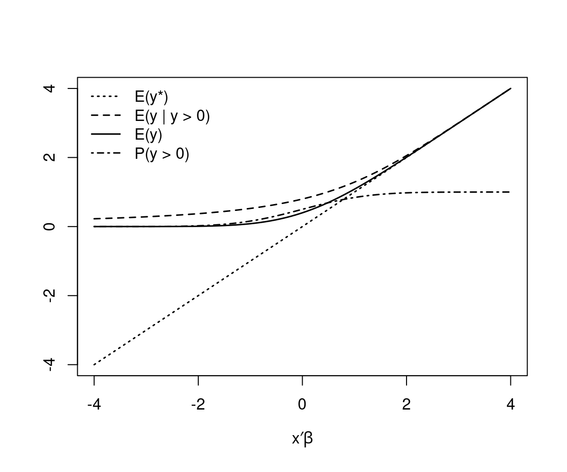
Figure 8.6: Expectation of the latent and the observed truncated variable
Marginal effects:
\[\begin{eqnarray*} \frac{\partial \text{P}(y > 0 ~|~ x)}{\partial x_l} & = & \phi(x^\top \beta / \sigma) \cdot \beta_l / \sigma\\[0.5cm] \frac{\partial \text{E}(y ~|~ y > 0,~ x)}{\partial x_l} & = & \beta_l \cdot \left[ 1 - \lambda(x^\top \beta / \sigma) ~ \{ x^\top \beta / \sigma ~+~ \lambda(x^\top \beta / \sigma) \}\right] \\[0.5cm] \frac{\partial \text{E}(y ~|~ x)}{\partial x_l} & = & \frac{\partial \text{P}(y > 0 ~|~ x)}{\partial x_l} \cdot \text{E}(y ~|~ y > 0,~ x) ~+~ \\ & & \text{P}(y > 0 ~|~ x) \cdot \frac{\partial \text{E}(y ~|~ y > 0,~ x)}{\partial x_l} \\ & = & \beta_l \cdot \Phi(x^\top \beta / \sigma) \\ \end{eqnarray*}\]
Remarks:
- Overall effect on \(\text{E}(y ~|~ x)\) is sum of an effect at the
- extensive margin (e.g., how much more likely a person is to join the labor force as education increases times the expected hours) and an effect at the
- intensive margin (e.g., how much the expected hours of work increase for workers as education increases times the probability of participation).
- OLS estimation (both for full and positive sample) is biased towards zero due to inability to capture non-constant marginal effects.
- Effects (e.g., at mean regressors) can again be considered instead of marginal effects.
Example: Effects in tobit model for PSID 1976 data (hand-crafted).
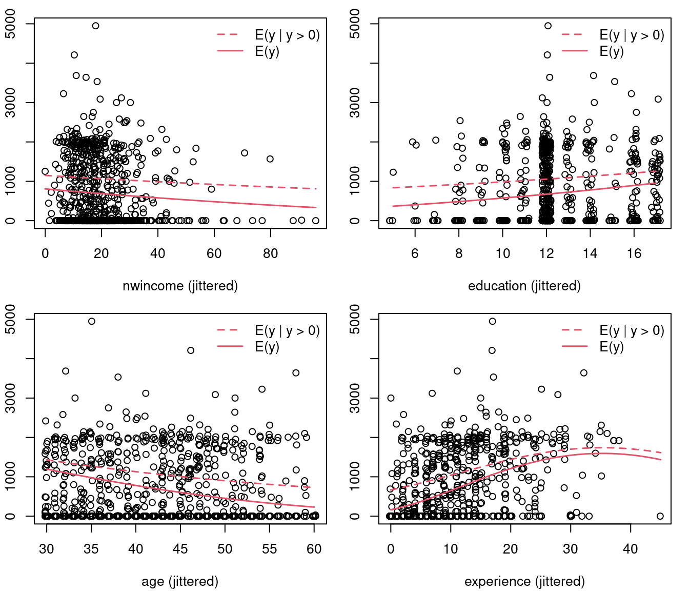
Figure 8.7: Effects in tobit model for PSID 1976 data (hand-crafted)
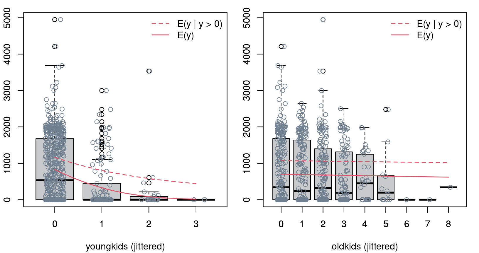
Figure 8.8: Effects of young- and old kids in tobit model for PSID 1976 data
Specification issues:
- The classical (uncensored) OLS regression model is rather robust to misspecifications of distributional form and even non-constant variances. Estimates remain consistent.
- In the tobit model, this is not the case. Misspecification of the likelihood (including constant variances) will lead to misspecification of the score. Hence, \(\text{E}(y ~ |~ y > 0,~ x)\) and \(\text{E}(y ~|~ x)\) are misspecified and estimates inconsistent.
- Crucial assumption: The same latent process drives the probability of a corner solution and the expectation of positive outcomes.
- Example: A single factor, such as number of old kids, can not increase the probability to work but decrease the expected number of hours conditional on participation in the labor force.
- Check for the latter: Cragg two-part model.
8.3 Cragg Two-Part Model
Idea: Similar to hurdle model for count data, employ two parts.
- Is \(y\) equal to zero or positive?
- If \(y > 0\), how large is \(y\)?
Formally: Likelihood has two separate parts.
- \(\text{P}(y > 0 ~|~ x)\): Binomial model (typically probit) for \(I(y > 0)\).
- \(\text{E}(y ~|~ y > 0,~ x)\): Truncated normal model for \(y\) given \(y > 0\).
Remarks:
- The tobit model is nested in the two-part model with probit link. Thus, LR tests etc. can be easily performed.
- If the tobit model is correctly specified, estimates from the probit model \(\hat \gamma\) would be consistent (but less efficient) for the scaled coefficients from the tobit model. Thus, \(\hat \beta / \hat \sigma\) should be similar to \(\hat \gamma\) in empirical samples.
In R: Employ separate modeling function. glm() with "probit" link can be used for selection part.
part_f <- update(hours_f, participation ~ .)
part_probit <- glm(part_f, data = PSID1976,
  family = binomial(link = "probit"))
coeftest(part_probit)
##
## z test of coefficients:
##
## Estimate Std. Error z value Pr(>|z|)
## (Intercept) 0.27007 0.50808 0.53 0.5950
## nwincome -0.01202 0.00494 -2.43 0.0149
## education 0.13090 0.02540 5.15 2.6e-07
## experience 0.12335 0.01876 6.58 4.8e-11
## I(experience^2) -0.00189 0.00060 -3.15 0.0017
## age -0.05285 0.00846 -6.25 4.2e-10
## youngkids -0.86833 0.11838 -7.34 2.2e-13
## oldkids 0.03601 0.04403 0.82 0.4135truncreg() from package truncreg (or trch() from package crch) can be employed for estimating the truncated normal regression model.
library("truncreg")
hours_trunc <- truncreg(hours_f, data = PSID1976,
  subset = participation == "yes")
coeftest(hours_trunc)
##
## z test of coefficients:
##
## Estimate Std. Error z value Pr(>|z|)
## (Intercept) 2055.713 461.265 4.46 8.3e-06
## nwincome -0.501 4.935 -0.10 0.91912
## education -31.270 21.796 -1.43 0.15139
## experience 73.007 20.229 3.61 0.00031
## I(experience^2) -0.970 0.581 -1.67 0.09521
## age -25.336 7.885 -3.21 0.00131
## youngkids -318.852 138.073 -2.31 0.02093
## oldkids -91.620 41.202 -2.22 0.02617
## sigma 822.479 39.320 20.92 < 2e-16Comparison of (scaled) parameter estimates from tobit, probit, and truncated model.
cbind("Censored"  = coef(hours_tobit) / hours_tobit$scale,
      "Threshold" = coef(part_probit),
      "Truncated" = coef(hours_trunc)[1:8] / coef(hours_trunc)[9])
## Censored Threshold Truncated
## (Intercept) 0.860327 0.270074 2.4994098
## nwincome -0.007856 -0.012024 -0.0006093
## education 0.071875 0.130904 -0.0380188
## experience 0.117256 0.123347 0.0887641
## I(experience^2) -0.001661 -0.001887 -0.0011788
## age -0.048488 -0.052852 -0.0308044
## youngkids -0.796795 -0.868325 -0.3876719
## oldkids -0.014454 0.036006 -0.1113943LR test and information criteria:
loglik <- c("Tobit" = logLik(hours_tobit),
  "Two-Part" = logLik(hours_trunc) + logLik(part_probit))
df <- c(9, 9 + 8)
-2 * loglik + 2 * df
## Tobit Two-Part
## 7656 7620## Tobit Two-Part
## 7698 7698## Two-Part
## 1.273e-08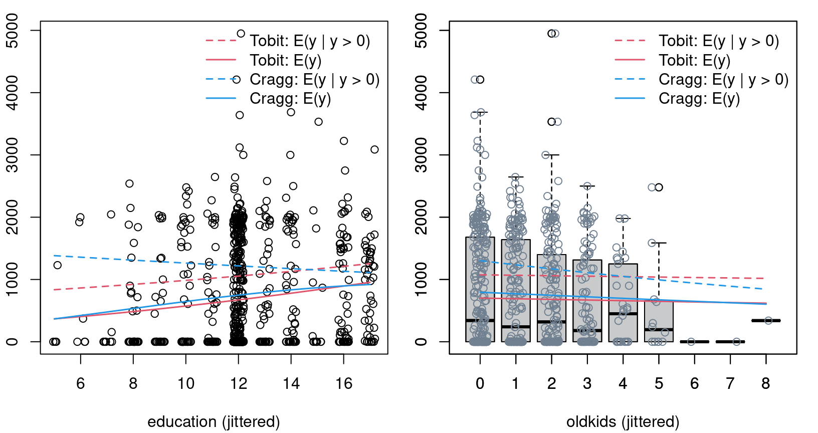
Figure 8.9: Education and oldkids effects in Tobit and Cragg model
8.4 Sample Selection Models
Idea: Employ censored regression model for observations \(y ~|~ y > c\) but model censoring threshold \(c\) as random variable.
Name: Incidental censoring or self selection.
Example: Distribution of wages.
- Wages are only observed for workers.
- Thus, the wages that non-workers would receive (if they decided to work) are unknown/latent.
- Individuals decide to work if their (possibly latent) offered wage \(w_0\) exceeds their individual reservation wage \(w_r\).
- The distribution of wages for workers are thus \(f(w_o ~|~ w_o > w_r)\) with random \(w_r\).
Formally: With \(y\) and \(c\) stochastic rewrite
\[\begin{equation*} f(y ~|~ y > c) ~=~ f(y ~|~ y - c > 0) ~=~ f(y_1 ~|~ y_2 > 0). \end{equation*}\]
Special cases:
- \(y_1 = y_2\): Standard censoring regression (i.e., tobit).
- \(y_1\) and \(y_2\) independent: \(f(y_1 ~|~ y_2 > 0) = f(y_1)\) (i.e., no selection).
Simple approach: Bivariate normal distribution for \((y_1, y_2)\) with correlation \(\varrho\), including special cases \(|\varrho| = 1\) (identity) and \(\varrho = 0\) (independence).
Alternatively: Employ different bivariate distribution or semiparametric approach.
Regression model: Employ (potentially overlapping) regressors for mean of both components.
\[\begin{eqnarray*} \mbox{Outcome equation:} & y_1 ~= & x^\top \beta ~+~ \varepsilon_1, \\ \mbox{Selection equation:} & y_2 ~= & z^\top \gamma ~+~ \varepsilon_2, \end{eqnarray*}\]
where
\[\begin{equation*} \left( \begin{array}{cc} \varepsilon_1 \\ \varepsilon_2 \end{array} \right) ~\sim~ \mathcal{N}\left( \left( \begin{array}{cc} 0 \\ 0 \end{array} \right), \left( \begin{array}{cc} \sigma^2 & \varrho \\ \varrho & 1 \end{array} \right) \right). \end{equation*}\]
Remarks:
- Observation rule: \(y_1\) is non-censored, observed for \(y_2 > 0\).
- In selection equation, only \(y_2 > 0\) vs. \(y_2 \le 0\) is observed. Hence, standardize \(\text{Var}(y_2) = 1\) for identifiability (as in probit model).
- Terminology: Heckman model, heckit model, sample selection model, self-selection model, tobit-2 model.
Conditional expectation:
\[\begin{equation*} \text{E}(y_1 ~|~ y_2 > 0,~ x) ~=~ x^\top \beta ~+~ \sigma \cdot \varrho \cdot \lambda(z^\top \gamma). \end{equation*}\]
Selection effect: Sample is
- positively selected for \(\varrho > 0\): \(\text{E}(y_1 ~|~ y_2 > 0,~ x) > \text{E}(y_1 ~|~ x)\),
- negatively selected for \(\varrho < 0\),
- and no selection occurs for \(\varrho = 0\).
Estimation:
- Efficient: Full maximum likelihood.
- Biased: OLS for non-censored observations.
- Consistent (and employed only for historical reasons): Two-step estimator. Probit model yielding \(\hat \gamma\) followed by OLS regressing \(y\) on \(x\) and \(\lambda(z^\top \hat \gamma)\).
Classical example: Estimation of mean wage offers (or worker’s productivity) from a sample of workers and wages.
In this context: Sample selection model called Gronau-Heckman-Roy model (by Winkelmann & Boes 2009) due to the authors that first recognized this problem and established its inference, respectively.
Identification: Economic considerations guide selection of variables \(x\) that affect the outcome and variables \(z\) that affect the selection.
- Typically, all variables \(x\) for the outcome also affect selection, especially in the case of “self selection”.
- Additional variables might affect the selection but not the outcome. Example: Presence of small children will affect selection but probably not the reservation wage.
- Such variables play a similar role as “instruments”.
Example: Female wages in PSID 1976 data. Employ semi-logarithmic wage equation with education and quadratic polynomial in experience.
OLS estimation: For selected subsample.
Sample selection model: Additionally employ age, number of old and young children, and other income as regressors in selection equation (corresponding to previously used part_f).
In R available in selection() from package sampleSelection:
Sample selection models
##
## z test of coefficients:
##
##                  Estimate Std. Error z value Pr(>|z|)
## (Intercept)      0.266449   0.508958    0.52   0.6006
## nwincome        -0.012132   0.004877   -2.49   0.0129
## education        0.131341   0.025382    5.17  2.3e-07
## experience       0.123282   0.018724    6.58  4.6e-11
## I(experience^2) -0.001886   0.000600   -3.14   0.0017
## age             -0.052829   0.008479   -6.23  4.7e-10
## youngkids       -0.867399   0.118651   -7.31  2.7e-13
## oldkids          0.035872   0.043475    0.83   0.4093
## (Intercept)     -0.552696   0.260379   -2.12   0.0338
## education        0.108350   0.014861    7.29  3.1e-13
## experience       0.042837   0.014879    2.88   0.0040
## I(experience^2) -0.000837   0.000417   -2.01   0.0449
## sigma            0.663398   0.022707   29.21  < 2e-16
## rho              0.026607   0.147078    0.18   0.8564
Interpretation: \(\hat \varrho\) is essentially zero signaling that there are no significant selection effects. Outcome part of Gronau-Heckman-Roy model and OLS for selected subsample are thus virtually identical.
##                 GHR (outcome) OLS (positive)
## (Intercept)        -0.5526963     -0.5220406
## education           0.1083502      0.1074896
## experience          0.0428368      0.0415665
## I(experience^2)    -0.0008374     -0.0008112
Similarly: Selection part of Gronau-Heckman-Roy model and probit for selection are thus virtually identical.
##                 GHR (selection) Probit (0 vs. positive)
## (Intercept)            0.266449                0.270074
## nwincome              -0.012132               -0.012024
## education              0.131341                0.130904
## experience             0.123282                0.123347
## I(experience^2)       -0.001886               -0.001887
## age                   -0.052829               -0.052852
## youngkids             -0.867399               -0.868325
## oldkids                0.035872                0.036006
Effects: Compare education effects graphically.
Set up auxiliary data with average regressor and varying education.
X <- model.matrix(hours_tobit)[, -c(1, 5)]
psid <- lapply(colnames(X), function(i)
  if(i != "education") mean(X[,i]) else
    seq(from = min(X[,i]), to = max(X[,i]), length = 100))
names(psid) <- colnames(X)
psid <- do.call("data.frame", psid)
Predictions for OLS:
Compute predictions for sample selection model by hand:
xb <- model.matrix(delete.response(terms(wage_f)),
  data = psid) %*% coef(wage_ghr, part = "outcome")
zg <- model.matrix(delete.response(terms(part_f)), data = psid) %*%
    head(coef(wage_ghr), 8)
wage_ghr_out <- xb + coef(wage_ghr)["sigma"] *
  coef(wage_ghr)["rho"] * dnorm(zg)/pnorm(zg)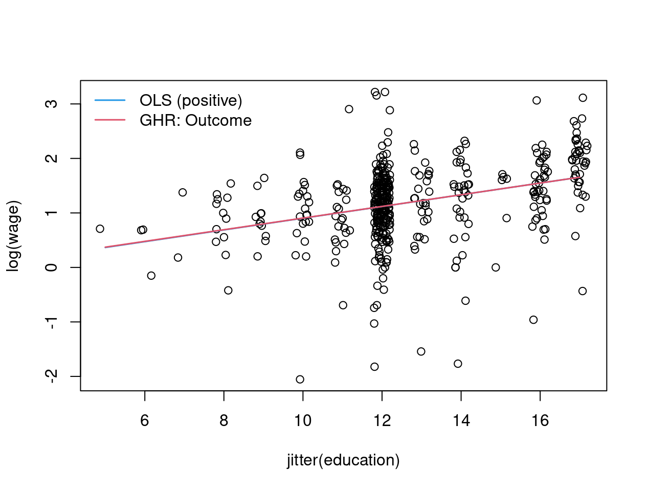
Figure 8.10: Sample selection model: education against log(wage) - jittered