Chapter 7 Count Data Models

7.1 Introduction

Examples: Typical economic examples for count data.

• Travel safety.
  \(y_i\): Number of accidents for airline \(i\) in last 10 years.
  Potential covariates: Economic indicators for airline, …
• Demand for recreation/leisure/travel.
  \(y_i\): Number of visits to recreational resort by person \(i\) in last year.
  Potential covariates: Income, costs, costs of alternatives.
• Health care utilization.
  \(y_i\): Number of doctor visits of person \(i\) in last year.
  Potential covariates: Age, gender, health, insurance, …
  
• Patents.
  \(y_i\): Number of patents of firm \(i\).
  Potential covariates: Expenditures for research & development, …

7.2 Poisson Distribution

Basic distribution: For \(y \in \mathbb{N}_0\) a natural model is Poisson distribution. If \(y \sim \mathit{Poisson}(\mu)\) with \(\mu > 0\), it has probability density function

\[\begin{equation*} f(y; \mu) ~=~ \frac{\exp(-\mu) \cdot \mu^y}{y!}. \end{equation*}\]

Properties:

• Moments: \(\text{E}(y) = \mu\), \(\text{Var}(y) = \mu\).
• Thus: Equidispersion.
• If \(y_1 \sim \mathit{Poisson}(\mu_1)\) and \(y_2 \sim \mathit{Poisson}(\mu_2)\) independently: \(y_1 + y_2 \sim \mathit{Poisson}(\mu_1 + \mu_2)\).
• If \(N \sim \mathit{Poisson}(\mu)\) and \(M ~|~ N \sim \mathit{Bin}(N, \pi)\): \(M \sim \mathit{Poisson}(\mu \cdot \pi)\).
• \(\text{P}(y = j) / \text{P}(y = j + 1) = (j+1) / \mu\) for \(j = 0, 1, \dots\).
• \(\partial \text{P}(y = j) / \partial \mu = (j - \mu) \cdot \text{P}(y = j) / \mu\).

Figure 7.1: Poisson probability distribution with different means

Background: Law of rare events.

Approximation: If \(Y_j \sim \mathit{Bin}(n, \pi_n)\), \(j = 1, \dots, n\), then \(Y := \sum_{j = 1}^n Y_j\) is approximately \(\mathit{Poisson}(\mu)\) with \(\mu = n \cdot \pi_n\) (for \(\pi_n\) “small” and \(n\) “large”).

Formally: For \(n \rightarrow \infty\) and \(\pi_n \rightarrow 0\) so that \(n \cdot \pi_n =: \mu\) constant,

\[\begin{equation*} \text{P}(Y = k) ~=~ {n \choose k} ~ \pi_n^k ~ (1 - \pi_n)^{n - k} ~\rightarrow~ \frac{\exp(-\mu) \cdot \mu^k}{k!}. \end{equation*}\]

Historical example: Von Bortkiewicz (1898), “Das Gesetz der kleinen Zahlen”. Data on number of deaths by horse or mule kicks in the years 1875–1894 in 10 (out of 14 reported) corps of the Prussian army.

Estimation: Mean \(\bar y\) is maximum likelihood estimator for \(\mu\).

Visualization: Observed and fitted (relative) frequencies. Preferably on square-root scale, also called rootogram.

data("HorseKicks", package = "vcd")
HorseKicks

## nDeaths
##   0   1   2   3   4 
## 109  65  22   3   1

mu <- weighted.mean(0:4, HorseKicks)
hk <- cbind(count = 0:4, freq = HorseKicks,
  rfreq = prop.table(HorseKicks), fit = dpois(0:4, mu))
hk

##   count freq rfreq      fit
## 0     0  109 0.545 0.543351
## 1     1   65 0.325 0.331444
## 2     2   22 0.110 0.101090
## 3     3    3 0.015 0.020555
## 4     4    1 0.005 0.003135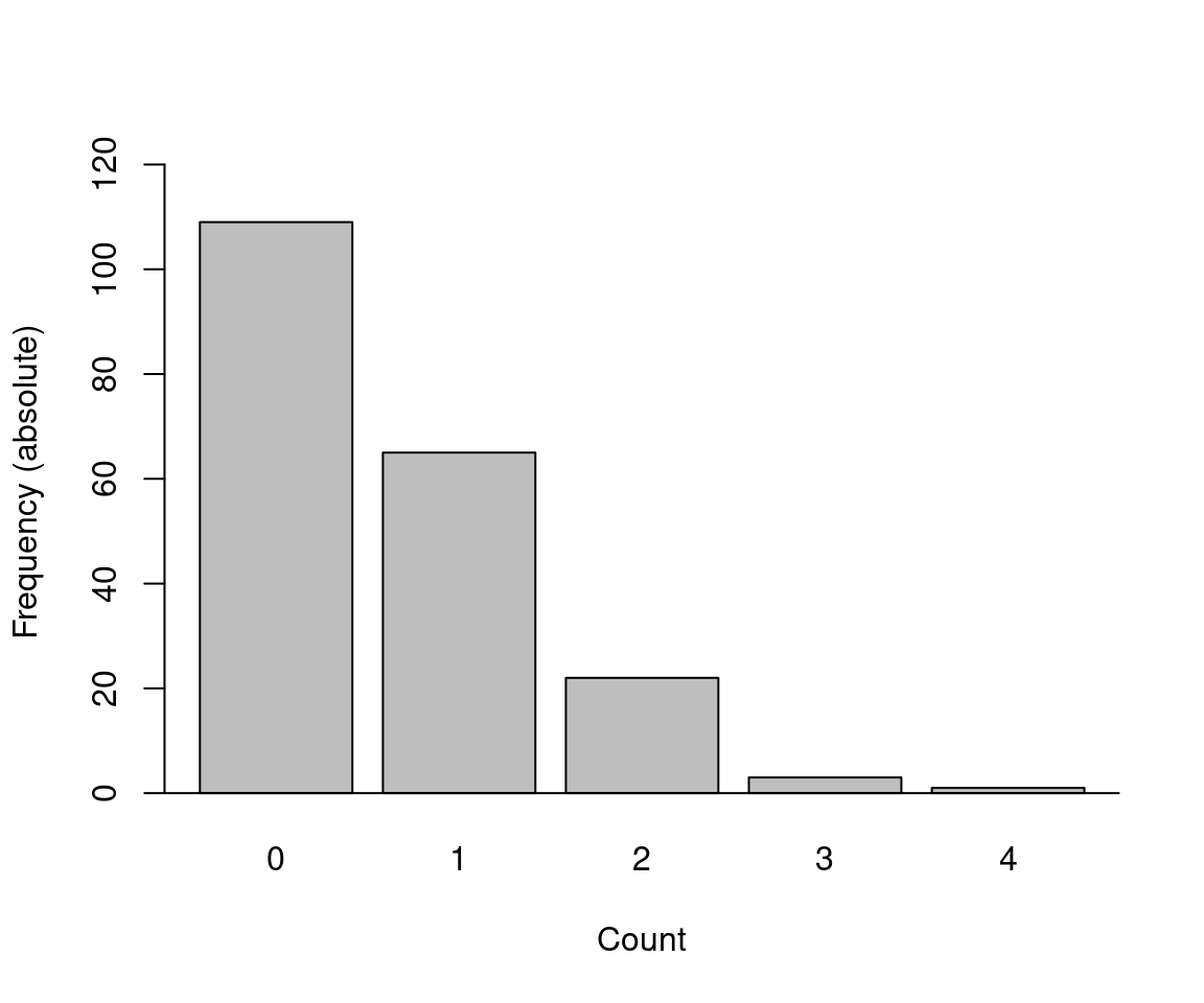

Figure 7.2: Absolute frequency - number of deaths by horse kicks

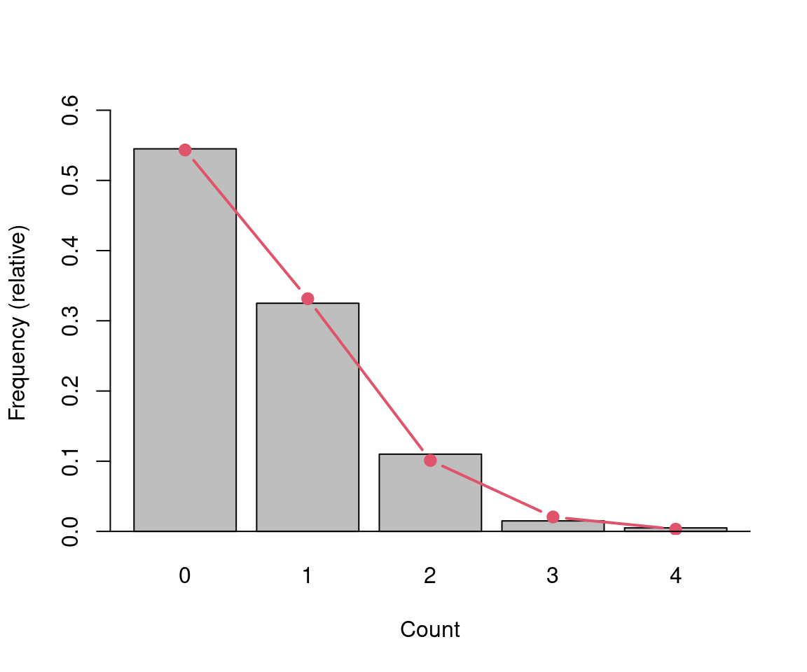
Figure 7.3: Relative frequency - number of deaths by horse kicks

barplot(sqrt(hk[,3]), ylim = c(-sqrt(0.005), sqrt(0.6)),
  xlab = "Count", ylab = "sqrt(Frequency)")
lines(x1, sqrt(hk[,4]), type = "b", lwd = 2, pch = 19, col = 2)
abline(h = 0)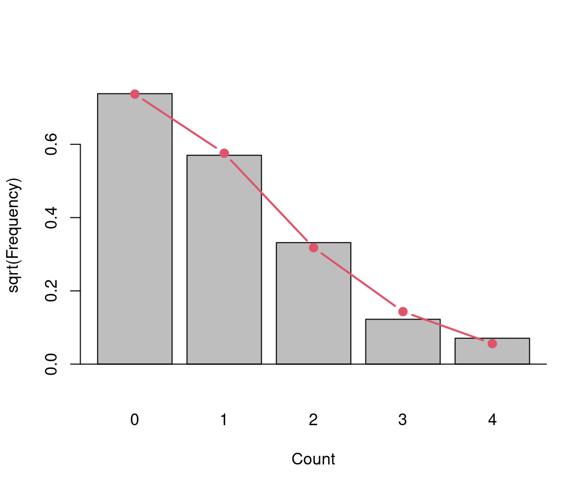

Figure 7.4: Square root of relative frequency - number of deaths by horse kicks

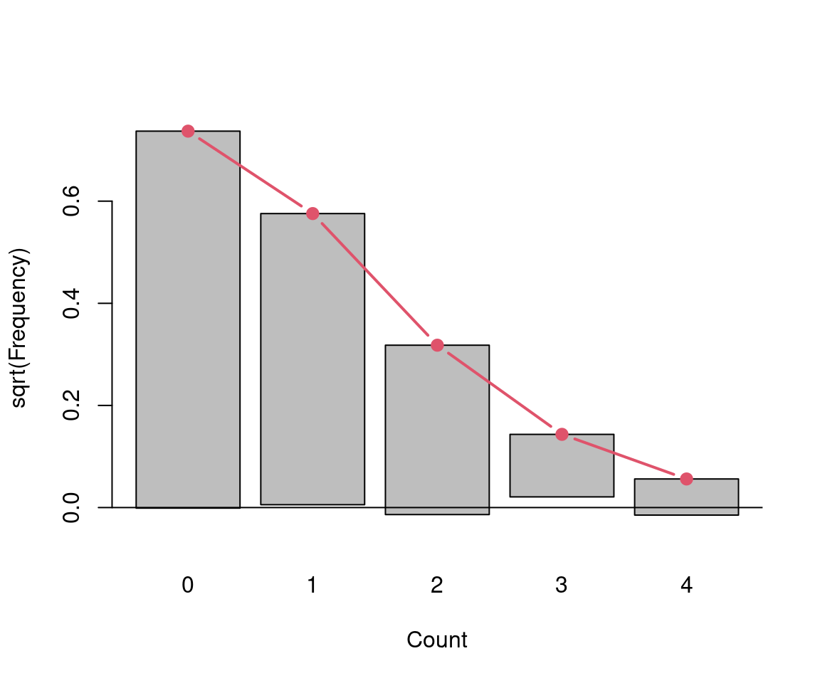
Figure 7.5: Hanging rootogram - number of deaths by horse kicks

7.3 Poisson GLM

Special case: Poisson distribution belongs to exponential family as

\[\begin{equation*} f(y; \mu) ~=~ \exp \left\{ y ~ \log(\mu) ~-~ \mu ~-~ \log(y!) \right\} \end{equation*}\]

Properties:

• Variance function is \(V(\mu) = \mu\) and the dispersion parameter is \(\phi = 1\) (signalling equidispersion).
• Natural parameter is \(\theta = \log(\mu)\), thus the canonical link is \(g(\mu) = \log(\mu)\).
• Hence, due to the resulting model equation

\[\begin{equation*} \log(\mu_i) = x_i^\top \beta \end{equation*}\] the Poisson GLM is also called log-linear model.

• \(\text{Var}(y_i ~|~ x_i) = \phi \cdot V(\mu_i) = \mu_i = \exp(x_i^\top \beta)\). Hence, the Poisson GLM is by construction heteroscedastic.

Estimation: Log-likelihood, score function, and Hessian.

\[\begin{eqnarray*} \ell(\beta) & = & \sum_{i = 1}^n \left\{ y_i ~ x_i^\top \beta ~-~ \exp(x_i^\top \beta) ~-~ \log(y_i!) \right\}, \\ s(\beta) & = & \sum_{i = 1}^n \left\{ y_i ~-~ \exp(x_i^\top \beta) \right\} ~ x_i, \\ H(\beta) & = & - \sum_{i = 1}^n \exp(x_i^\top \beta) ~ x_i x_i^\top ~=~ -X^\top \Omega(\beta) X, \end{eqnarray*}\]

where \(\Omega(\beta) = \text{diag}(\exp(x_i^\top \beta))\), i.e., negative definite. Thus, log-likelihood is globally concave. As the Hessian is independent of \(y\), observed and expected Hessian coincide.

Marginal effects:

\[\begin{eqnarray*} \frac{\partial \text{E}(y_i ~|~ x_i)}{\partial x_{il}} ~=~ \frac{\partial \exp(x_i^\top \beta)}{\partial x_{il}} ~=~ \exp(x_i^\top \beta) \cdot \beta_l. \end{eqnarray*}\]

Discrete changes:

\[\begin{equation*} \frac {\text{E}(y_i ~|~ x_1)}{\text{E}(y_i ~|~ x_2)} ~=~ \exp \{ (x_1 - x_2)^\top \beta \}. \end{equation*}\]

Thus, for a single unit change \(x_1 = x_2 + \Delta x_{2l}\) for a “small” \(\beta_l\) this is approximately \(1 + \beta_l\). This corresponds to a relative change of approximately \(100 \cdot \beta_l\)%.

7.3.1 Example: Recreation demand

Cross-section data on the number of recreational boating trips to Lake Somerville, Texas, in 1980, based on a survey administered to 2,000 registered leisure boat owners in 23 counties in eastern Texas.

A data frame containing 659 observations on 8 variables:

Table 7.1: Variables in the Recreation demand data set

Variable	Description
trips	Number of recreational boating trips.
quality	Facility’s subjective quality ranking on scale 1–5.
ski	Was the individual engaged in water-skiing?
income	Annual household income (in 1,000 USD).
userfee	Did the owner pay an annual user fee at Lake Somerville?
costC	Expenditure when visiting Lake Conroe (in USD).
costS	Expenditure when visiting Lake Somerville (in USD).
costH	Expenditure when visiting Lake Houston (in USD).

data("RecreationDemand", package = "AER")
summary(RecreationDemand)

##      trips          quality      ski          income     userfee  
##  Min.   : 0.00   Min.   :0.00   no :417   Min.   :1.00   no :646  
##  1st Qu.: 0.00   1st Qu.:0.00   yes:242   1st Qu.:3.00   yes: 13  
##  Median : 0.00   Median :0.00             Median :3.00            
##  Mean   : 2.24   Mean   :1.42             Mean   :3.85            
##  3rd Qu.: 2.00   3rd Qu.:3.00             3rd Qu.:5.00            
##  Max.   :88.00   Max.   :5.00             Max.   :9.00            
##      costC           costS           costH      
##  Min.   :  4.3   Min.   :  4.8   Min.   :  5.7  
##  1st Qu.: 28.2   1st Qu.: 33.3   1st Qu.: 29.0  
##  Median : 41.2   Median : 47.0   Median : 42.4  
##  Mean   : 55.4   Mean   : 59.9   Mean   : 56.0  
##  3rd Qu.: 69.7   3rd Qu.: 72.6   3rd Qu.: 68.6  
##  Max.   :493.8   Max.   :491.5   Max.   :491.0

7.3.2 Recreation demand: Visualization

Univariate visualization: Histogram or bar plot of discrete count response.

plot(table(RecreationDemand$trips))
hist(RecreationDemand$trips, breaks = 0:90 - 0.5)

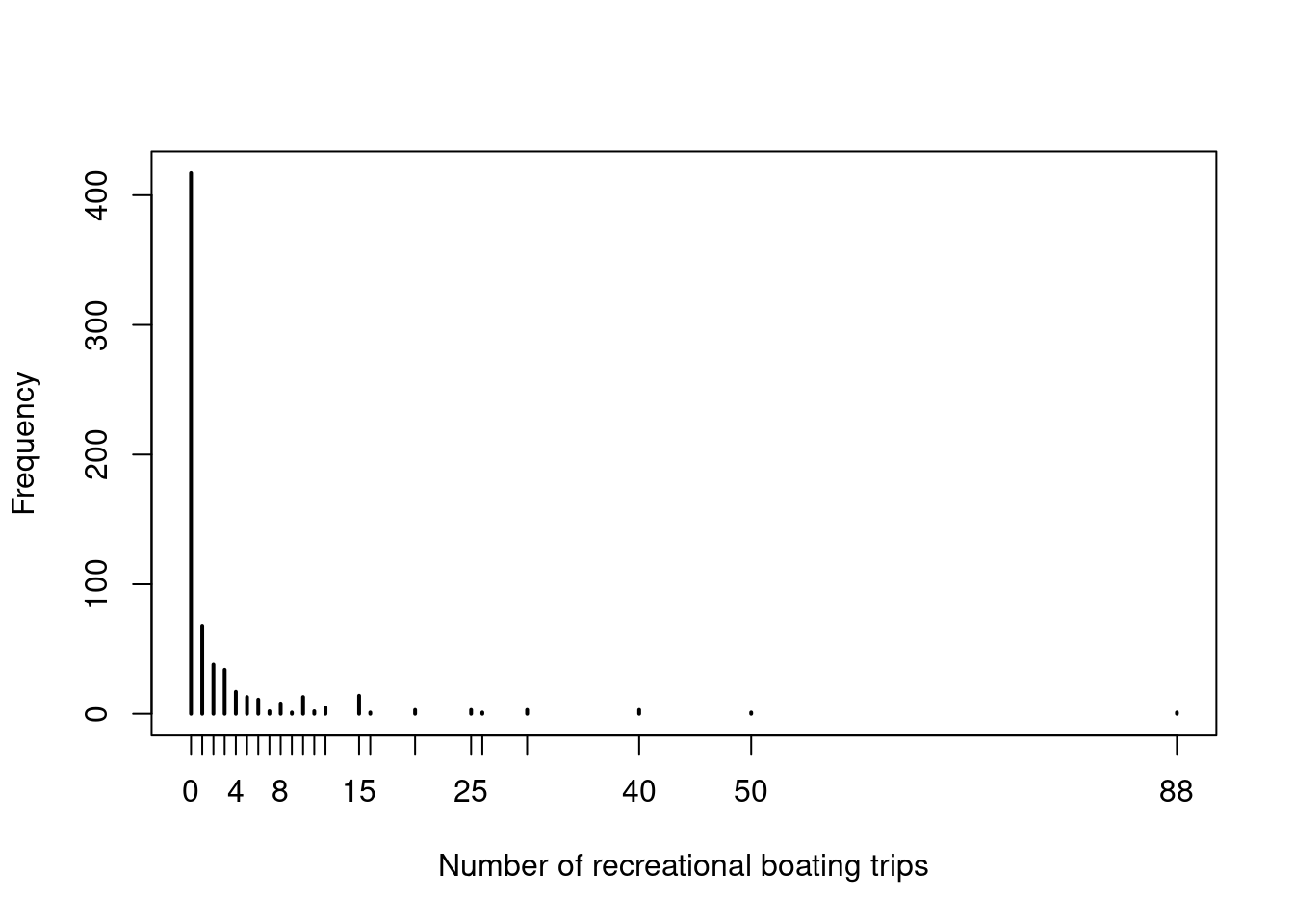
Figure 7.6: Absolute frequency - Number of trips

Bivariate visualization: Standard scatter plots do not work well due to many ties; employ discretized version in spine plots/spinograms instead.

trips1 <- cut(RecreationDemand$trips, 
  breaks = c(0:2, 4, 8, 90) - 0.5,
  labels = c("0", "1", "2-3", "4-7", "8+"))
plot(trips1 ~ ski, data = RecreationDemand)
plot(trips1 ~ quality, data = RecreationDemand,
  breaks = 0:6 - 0.5)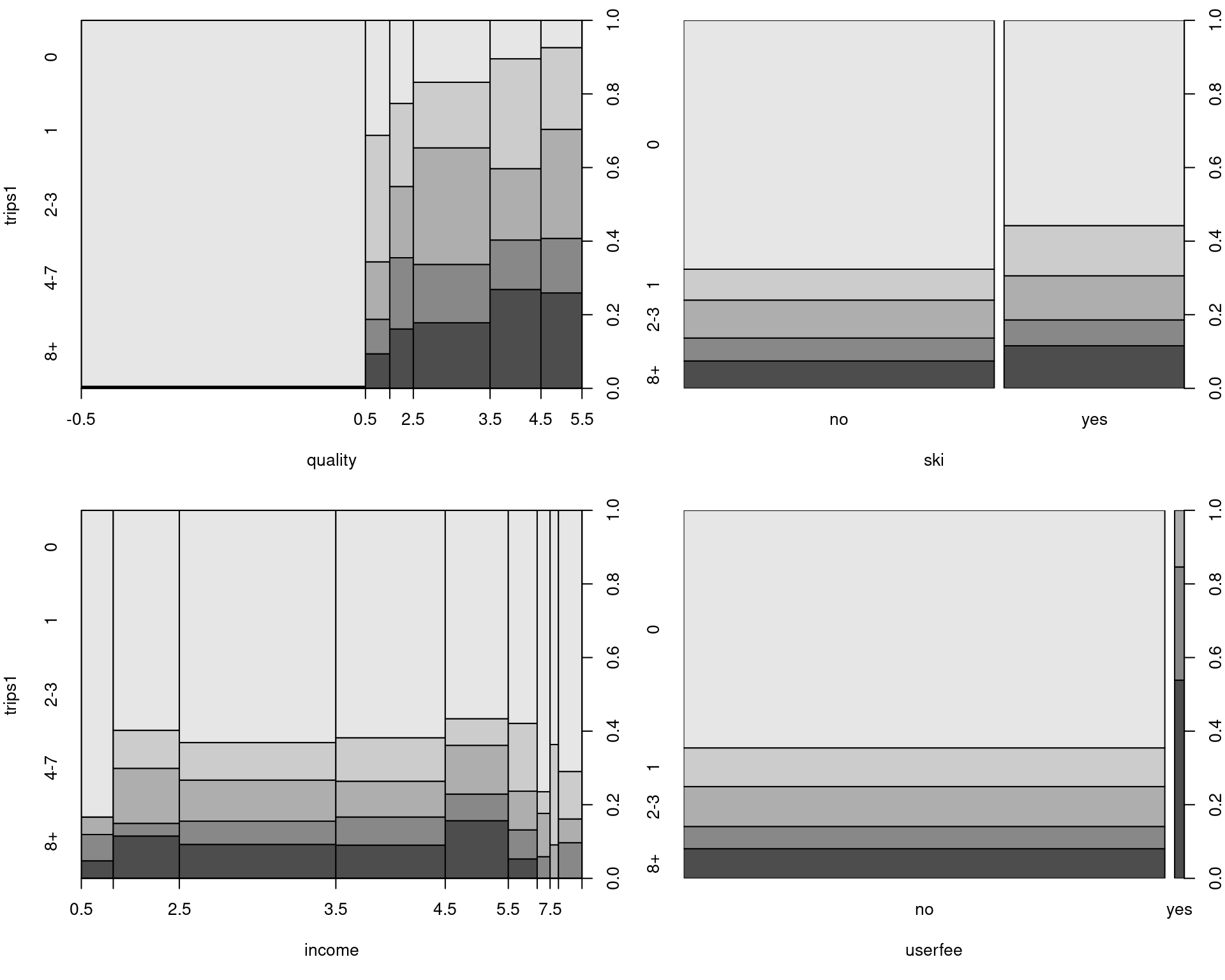

Figure 7.7: Spine plots: trips vs. quality, ski, income and userfee

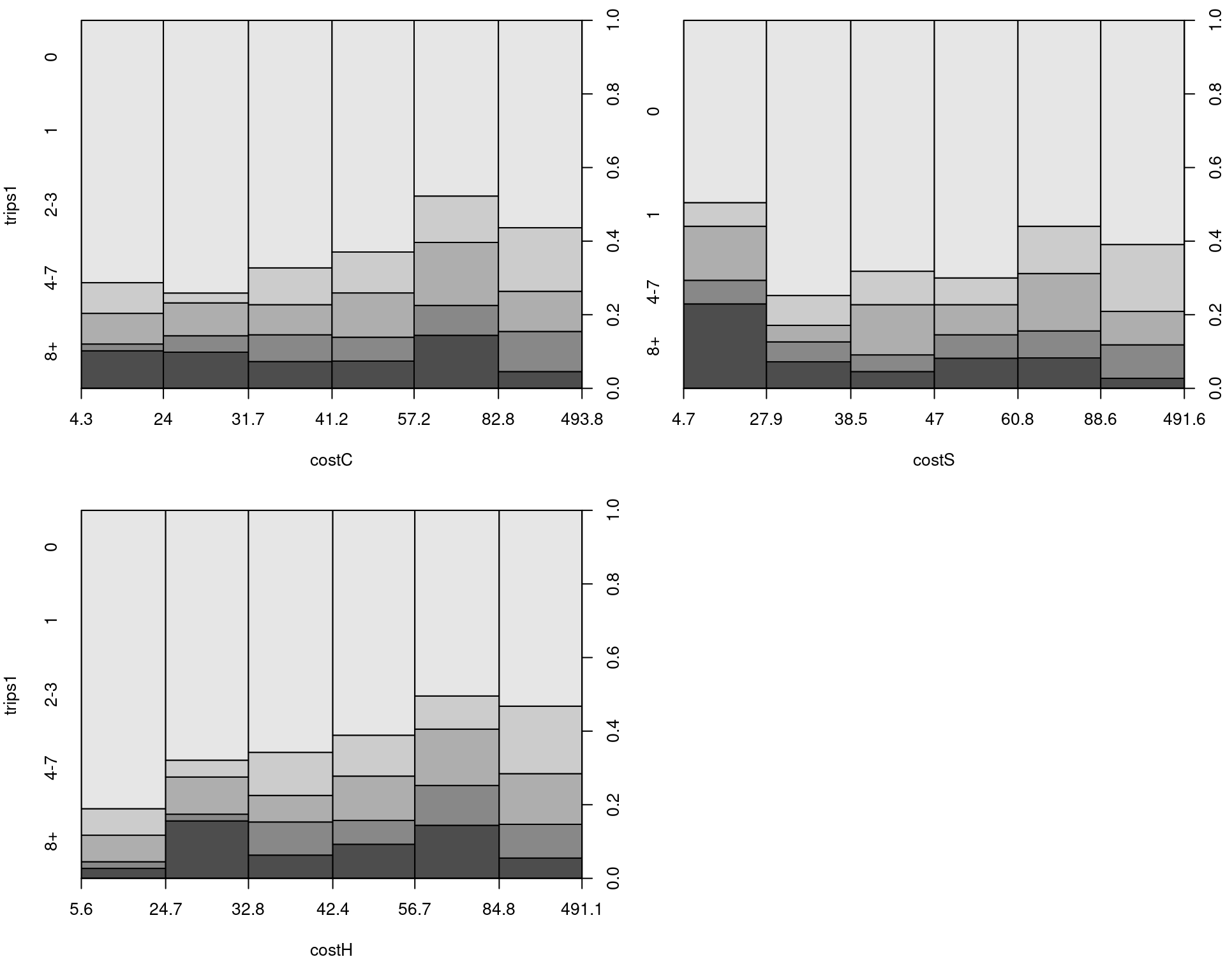
Figure 7.8: Spine plots: trips vs. cost variables

Sometimes continuity-corrected log-response log(y + 0.5) works well, jittered if necessary.

7.3.3 Recreation demand: Poisson GLM

rd_pois <- glm(trips ~ ., data = RecreationDemand,
  family = poisson)
summary(rd_pois)

## 
## Call:
## glm(formula = trips ~ ., family = poisson, data = RecreationDemand)
## 
## Coefficients:
##             Estimate Std. Error z value Pr(>|z|)
## (Intercept)  0.26499    0.09372    2.83   0.0047
## quality      0.47173    0.01709   27.60  < 2e-16
## skiyes       0.41821    0.05719    7.31  2.6e-13
## income      -0.11132    0.01959   -5.68  1.3e-08
## userfeeyes   0.89817    0.07899   11.37  < 2e-16
## costC       -0.00343    0.00312   -1.10   0.2713
## costS       -0.04254    0.00167  -25.47  < 2e-16
## costH        0.03613    0.00271   13.34  < 2e-16
## 
## (Dispersion parameter for poisson family taken to be 1)
## 
##     Null deviance: 4849.7  on 658  degrees of freedom
## Residual deviance: 2305.8  on 651  degrees of freedom
## AIC: 3075
## 
## Number of Fisher Scoring iterations: 7

Effects:

library("effects")
rd_eff <- allEffects(rd_pois,
  xlevels = list(costC = 0:250, costS = 0:250, costH = 0:250))
plot(rd_eff, rescale.axis = FALSE)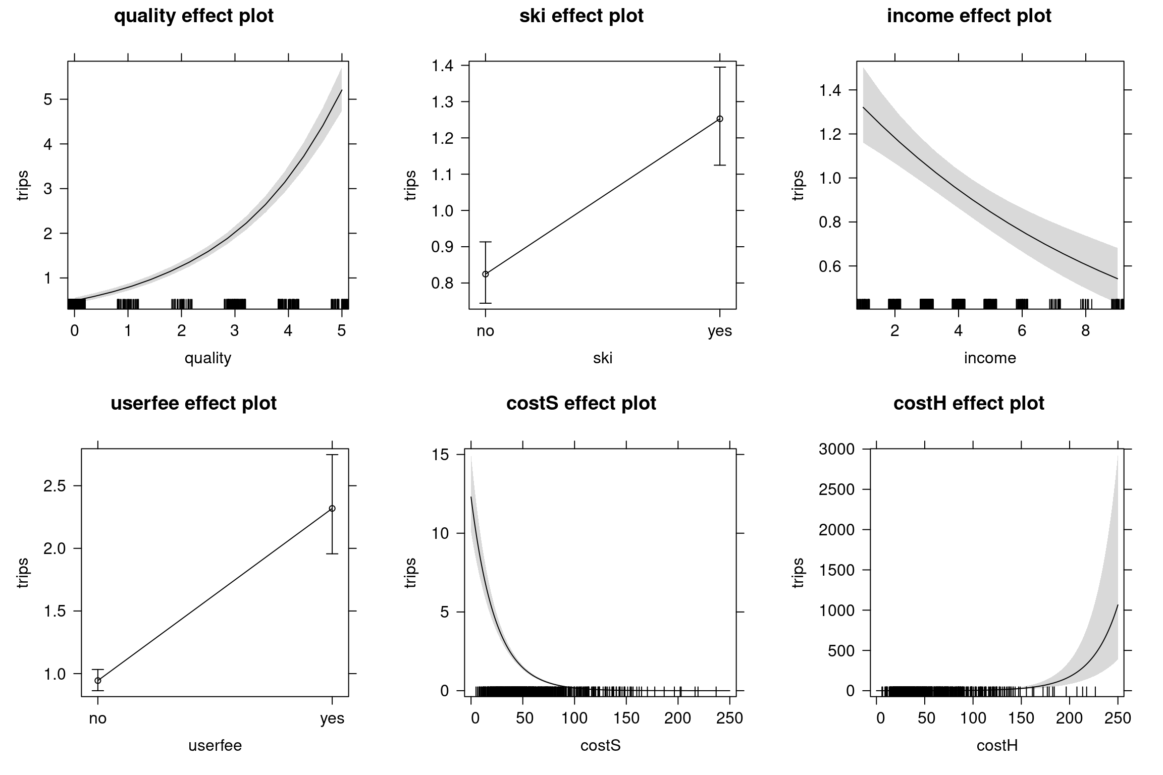

Figure 7.9: Recreation demand effect plots

Log-likelihood:

logLik(rd_pois)

## 'log Lik.' -1529 (df=8)

Goodness of fit: Here, graphical assessment of observed frequencies and expected frequencies \(\sum_{i = 1}^n \widehat{\text{P}}(y_i = j) = \sum_{i = 1}^n f(j; \hat \mu_i)\) in hanging rootogram. E.g., for \(j = 0\)

table(trip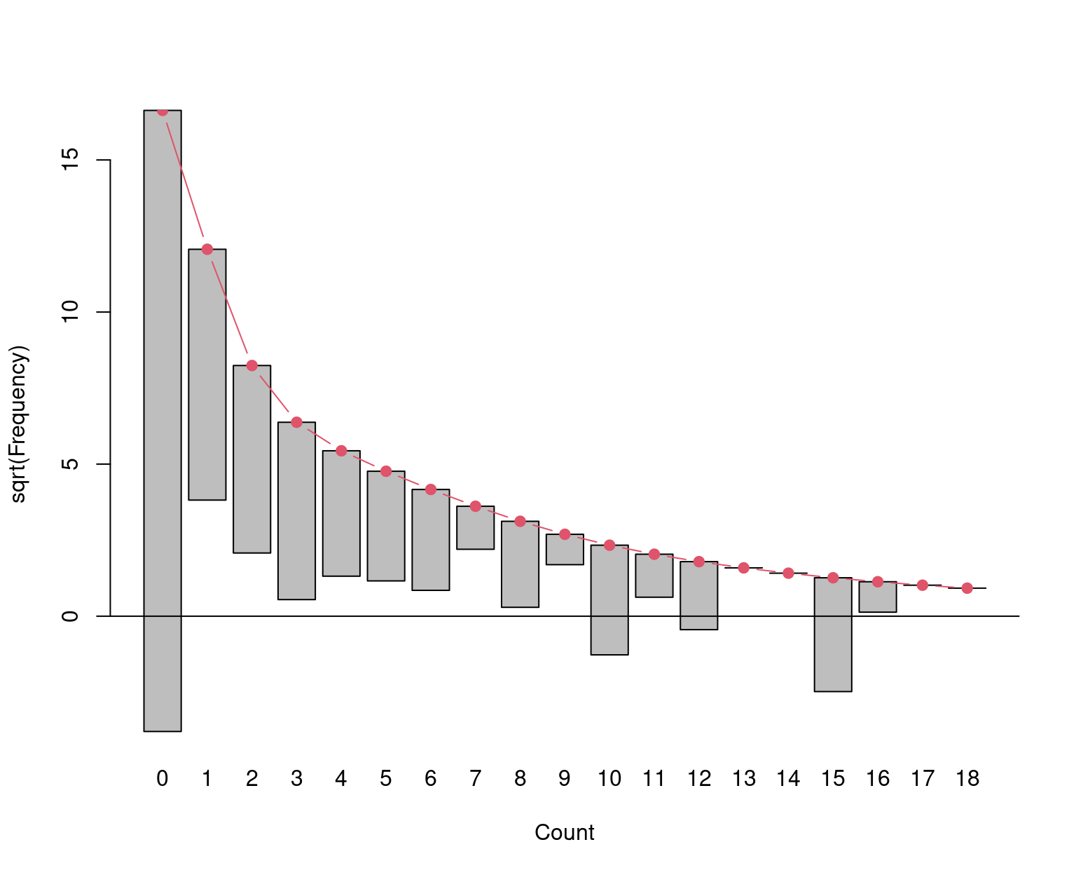s1)[1]

##   0 
## 417

sum(dpois(0, fitted(rd_pois)))

## [1] 276.5

Figure 7.10: Recreation demand: Hanging rootogram

Typical problem: Poisson GLM is often no suitable probability model.

Excess zeros: Response has 63.28% zeros, much more than captured by a Poisson regression.

head(prop.table(table(RecreationDemand$trips)))

## 
##       0       1       2       3       4       5 
## 0.63278 0.10319 0.05766 0.05159 0.02580 0.01973

mean(dpois(0, fitted(rd_pois)))

## [1] 0.4196

Overdispersion: Variance is often (much) larger than mean.

with(RecreationDemand, var(trips)/mean(trips))

## [1] 17.64

(Note, however, that this does not consider the influence of covariables.)

7.4 Overdispersion and Unobserved Heterogeneity

7.4.1 Overdispersion

Problem: In many applications (in economics and the social sciences) \(\text{Var}(y_i ~|~ x_i) > \text{E}(y_i ~|~ x_i)\).

Consequences: If ignored, point estimates from a Poisson model may or may not be valid (depending on correct specification of the mean equation, see below). However, inference is biased due to incorrect estimates of the covariance matrix (i.e., also the standard errors).

Solutions: Consider more general \(\text{Var}(y_i ~|~ x_i)\).

• Quasi-Poisson: Employ Poisson model for the mean equation but allow overdispersion in variance equation.
• Robust covariances: Employ Poisson model for the mean equation but leave rest of the likelihood unspecified. Estimate covariances under general heteroscedasticity.
• Negative binomial: Employ more general likelihood (both for mean and variance) that allows for overdispersion.

Test: To test for over- (or under-)dispersion, consider the specification

\[\begin{equation*} \text{Var}(y_i ~|~ x_i) ~=~ \mu_i ~+~ \alpha \cdot h(\mu_i), \end{equation*}\]

where \(h(\mu)\) is a positive function, e.g.,

\[\begin{equation*} h(\mu) ~=~ \left\{ \begin{array}{ll} \mu^2 & \mbox{corresponding to negative binomial NB2 model,}\\ \mu & \mbox{corresponding to negative binomial NB1 model.} \end{array} \right. \end{equation*}\]

Then, equidispersion corresponds to \(\alpha = 0\), underdispersion to \(\alpha < 0\), and overdispersion to \(\alpha > 0\). \(\alpha\) can be estimated and tested using an auxiliary regression based on adjusted squared Pearson residuals.

Note: However, overdispersion can be relevant (for the inference in the Poisson GLM) before it is significant in a formal test. Thus, if in doubt, do not rely on equidispersion.

Example: Test for overdispersion in rd_pois using \(h(\mu) = \mu^2\) (NB2) alternative.

dispersiontest(rd_pois, trafo = 2)

## 
##  Overdispersion test
## 
## data:  rd_pois
## z = 2.9, p-value = 0.002
## alternative hypothesis: true alpha is greater than 0
## sample estimates:
## alpha 
## 1.316

Example: Test for overdispersion in rd_pois using \(h(\mu) = \mu\) (NB1) alternative.

dispersiontest(rd_pois, trafo = 1)

## 
##  Overdispersion test
## 
## data:  rd_pois
## z = 2.4, p-value = 0.008
## alternative hypothesis: true alpha is greater than 0
## sample estimates:
## alpha 
## 5.566

Example: Test for overdispersion in rd_pois using \(h(\mu) = \mu\) (NB1) alternative. Reparametrize \(\phi = 1 + \alpha\).

dispersiontest(rd_pois)

## 
##  Overdispersion test
## 
## data:  rd_pois
## z = 2.4, p-value = 0.008
## alternative hypothesis: true dispersion is greater than 1
## sample estimates:
## dispersion 
##      6.566

7.4.2 Quasi-Poisson GLM

Formally: Test idea can be turned into a formal model.

• The score function for \(\beta\) (and thus the estimating equations and mean function) are assumed to be correct.
• Relax remaining likelihood to allow overdispersion.

\[\begin{eqnarray*} \text{E}(y_i ~|~ x_i) & = & \exp(x_i^\top \beta) \\ \text{Var}(y_i ~|~ x_i) & = & \phi \cdot V(\mu_i) ~=~ \phi \cdot \mu_i, \end{eqnarray*}\]

where \(\phi\) is not constrained to \(1\).

Properties:

• This is called quasi-Poisson model in the GLM literature.
• The quasi-ML estimator coincides with the ML estimator \(\hat \beta\) because the score function is unchanged.
• The model is not associated with a likelihood. Conditional mean but not conditional probability model.
• Estimate \(\hat \phi\) required for inference.

Typically: Estimate \(\phi\) from (some version of) residuals.

\[\begin{equation*} \hat \phi ~=~ \frac{1}{n-k} \sum_{i = 1}^n r_i^2, \end{equation*}\]

where \(r_i\) could be the Pearson or deviance residuals. But other versions of estimators exist. Hence, indicate estimator in empirical applications.

In R: A quasipoisson family to be plugged into glm() is provided. By default, it uses the Pearson residuals \(r_i = (y_i - \hat \mu_i) / \sqrt{\hat \mu_i}\) in the above estimator \(\hat \phi\).

rd_qpois <- glm(trips ~ ., data = RecreationDemand,
  family = quasipoisson)

summary(rd_qpois)

## 
## Call:
## glm(formula = trips ~ ., family = quasipoisson, data = RecreationDemand)
## 
## Coefficients:
##             Estimate Std. Error t value Pr(>|t|)
## (Intercept)  0.26499    0.23521    1.13   0.2603
## quality      0.47173    0.04289   11.00  < 2e-16
## skiyes       0.41821    0.14353    2.91   0.0037
## income      -0.11132    0.04916   -2.26   0.0239
## userfeeyes   0.89817    0.19822    4.53  7.0e-06
## costC       -0.00343    0.00782   -0.44   0.6613
## costS       -0.04254    0.00419  -10.15  < 2e-16
## costH        0.03613    0.00680    5.31  1.5e-07
## 
## (Dispersion parameter for quasipoisson family taken to be 6.298)
## 
##     Null deviance: 4849.7  on 658  degrees of freedom
## Residual deviance: 2305.8  on 651  degrees of freedom
## AIC: NA
## 
## Number of Fisher Scoring iterations: 7

logLik(rd_qpois)

## 'log Lik.' NA (df=9)

sum(residuals(rd_qpois, type = "pearson")^2) /
  df.residual(rd_qpois)

## [1] 6.298

7.4.3 Sandwich covariances

Similar idea: As before, assume that score function for \(\beta\) is correctly specified but remaining likelihood is not. Now allow general patterns of heteroscedasticity by means of sandwich covariance matrix estimate (or “robust” standard errors).

For correctly specified ML: Information matrix equality holds (under regularity conditions). Observed/expected information and outer product of gradients coincide.

\[\begin{eqnarray*} \text{Var}(\hat \beta ~|~ X) & = & \frac{1}{n} A_0^{-1} ~=~ \left( \sum_{i = 1}^n \mu_i x_i x_i^\top \right)^{-1} \\ & = & \frac{1}{n} B_0^{-1} ~=~ \left\{ \sum_{i = 1}^n \text{E}[(y_i - \mu_i) ~ x_i ~ ((y_i - \mu_i) ~ x_i)^\top ~|~ X] \right\}^{-1} \\ & & \phantom{\frac{1}{n} B_0^{-1}} ~=~ \left\{ \sum_{i = 1}^n \text{E}[(y_i - \mu_i)^2 ~|~ X] ~ x_i x_i^\top \right\}^{-1} \end{eqnarray*}\]

Under misspecification: To account for potential misspecifications of the remaining likelihood – including but not limited to \(\text{E}(y_i ~|~ x_i) \neq \text{Var}(y_i ~|~ x_i)\) – employ sandwich estimator:

\[\begin{eqnarray*} \hat A^{-1} \hat B \hat A^{-1} & = & \left( \sum_{i = 1}^n \hat \mu_i x_i x_i^\top \right)^{-1} \left( \sum_{i = 1}^n (y_i - \hat \mu_i)^2 x_i x_i^\top \right) \left( \sum_{i = 1}^n \hat \mu_i x_i x_i^\top \right)^{-1} \\ & \rightarrow & A_0^{-1} B_0 A_0^{-1} \end{eqnarray*}\] under regularity conditions.

modelsummary(list("Poisson sandwich vcov" = rd_pois), 
             vcov=sandwich, fmt=3, estimate="{estimate}{stars}")

	Poisson sandwich vcov
(Intercept)	0.265
	(0.432)
quality	0.472***
	(0.049)
skiyes	0.418*
	(0.194)
income	-0.111*
	(0.050)
userfeeyes	0.898***
	(0.247)
costC	-0.003
	(0.015)
costS	-0.043***
	(0.012)
costH	0.036***
	(0.009)
Num.Obs.	659
AIC	3074.9
BIC	3110.8
Log.Lik.	-1529.431
RMSE	6.09
Std.Errors	Custom

Note that ski and income are not significant at 1% level anymore.

Comparison: All methods employ same conditional mean model and lead to same \(\hat \beta\). Only estimated covariances differ.

round(sqrt(cbind(
  "Poisson"       = diag(vcov(rd_pois)),
  "Quasi-Poisson" = diag(vcov(rd_qpois)),
  "Sandwich"      = diag(sandwich(rd_pois))
)), digits = 3)

##             Poisson Quasi-Poisson Sandwich
## (Intercept)   0.094         0.235    0.432
## quality       0.017         0.043    0.049
## skiyes        0.057         0.144    0.194
## income        0.020         0.049    0.050
## userfeeyes    0.079         0.198    0.247
## costC         0.003         0.008    0.015
## costS         0.002         0.004    0.012
## costH         0.003         0.007    0.009

Here, quasi-Poisson and sandwich standard errors are similar, but Poisson standard errors are much too small.

7.4.4 Unobserved heterogeneity

Question: What are the (potential) sources of overdispersion?

Answer: Unobserved heterogeneity. Not all relevant regressors are known, some remaining deviations \(\varepsilon_i\) with mean 0 cannot be observed. The mean is then

\[\begin{equation*} \tilde \mu_i ~=~ \exp(x_i^\top \beta ~+~ \varepsilon_i) ~=~ \mu_i ~ \nu_i, \end{equation*}\]

where \(\nu_i = \exp(\varepsilon_i)\) with \(E(\nu_i ~|~ x_i) = 1\) and \(\text{Var}(\nu_i ~|~ x_i) = \alpha\).

This implies:

\[\begin{eqnarray*} \text{E}(y_i ~|~ x_i) & = & \text{E}(\tilde \mu_i ~|~ x_i) ~=~ \mu_i ~ E(\nu_i ~|~ x_i) ~=~ \mu_i,\\ \text{Var}(y_i ~|~ x_i) & = & \text{E}(\tilde \mu_i ~|~ x_i) ~+~ \text{Var}(\tilde \mu_i ~|~ x_i) ~=~ \mu_i ~+~ \alpha \cdot \mu_i^2, \end{eqnarray*}\]

justifying the previously considered variance equations.

Conditional distribution: To obtain the full distribution (rather than the first two moments only), the full distribution \(w(\nu_i ~|~ x_i)\) needs to be known. Then, influence of \(u_i\) can be integrated out.

\[\begin{equation*} f(y_i ~|~ x_i) ~=~ \int_0^\infty f(y_i ~|~ x_i, \nu_i) ~ w(\nu_i ~|~ x_i) ~d \nu_i \end{equation*}\]

which corresponds to a continuous mixture distribution.

Question: What are useful assumptions for \(w(\nu_i ~|~ x_i)\)?

Answer: Preferably such that there is a closed form solution for \(f(y_i ~|~ x_i)\). For extending the Poisson distribution, a gamma mixture is often employed.

Properties: If \(x \sim \mathit{Gamma}(\gamma, \theta)\) with \(\gamma, \theta > 0\),

\[\begin{equation*} w(x; \gamma, \theta) ~=~ \frac{\theta^\gamma}{\Gamma(\gamma)} ~ x^{\gamma-1} ~ \exp(-\theta x), \end{equation*}\]

with \(\text{E}(x) = \gamma/\theta\) and \(\text{Var}(x) = \gamma/\theta^2\).

Note: \(\Gamma(\cdot)\) is the gamma function

\[\begin{equation*} \Gamma(\gamma) ~= ~ \int_0^\infty z^{\gamma-1} \exp(-z) ~d z. \end{equation*}\] It is a generalization of the factorial function. For integer-valued \(y\): \(\Gamma(y+1) = y!\).

Here: Employ \(\nu_i \sim \mathit{Gamma}(\theta, \theta)\) so that \(\text{E}(\nu_i) = 1\). Then \(\text{Var}(\nu_i) = 1/\theta\), i.e., \(\alpha = 1/\theta\) in the generic notation.

Now: Continuous mixture of Poisson distribution \(h(y; \tilde \mu)\) with gamma weights. This is called negative binomial distribution. It can be shown that

\[\begin{eqnarray*} f(y; \mu, \theta) & = & \int_0^\infty h(y; \mu \nu) ~ w(\nu; \theta, \theta) ~d \nu \\ & = & \frac{\Gamma(y + \theta)}{\Gamma(\theta) \cdot y!} \cdot \frac{\mu^{y} \cdot \theta^\theta}{(\mu + \theta)^{y + \theta}}, \end{eqnarray*}\]

which has \(\text{E}(y) = \mu\) and \(\text{Var}(y) = \mu + 1/\theta \cdot \mu^2\).

Special cases:

• Poisson: \(\theta = \infty\).
• Geometric: \(\theta = 1\).

7.4.5 Poisson vs. negative binomial distribution

Again, the probability distribution function of the Poisson distribution with different means looks the following: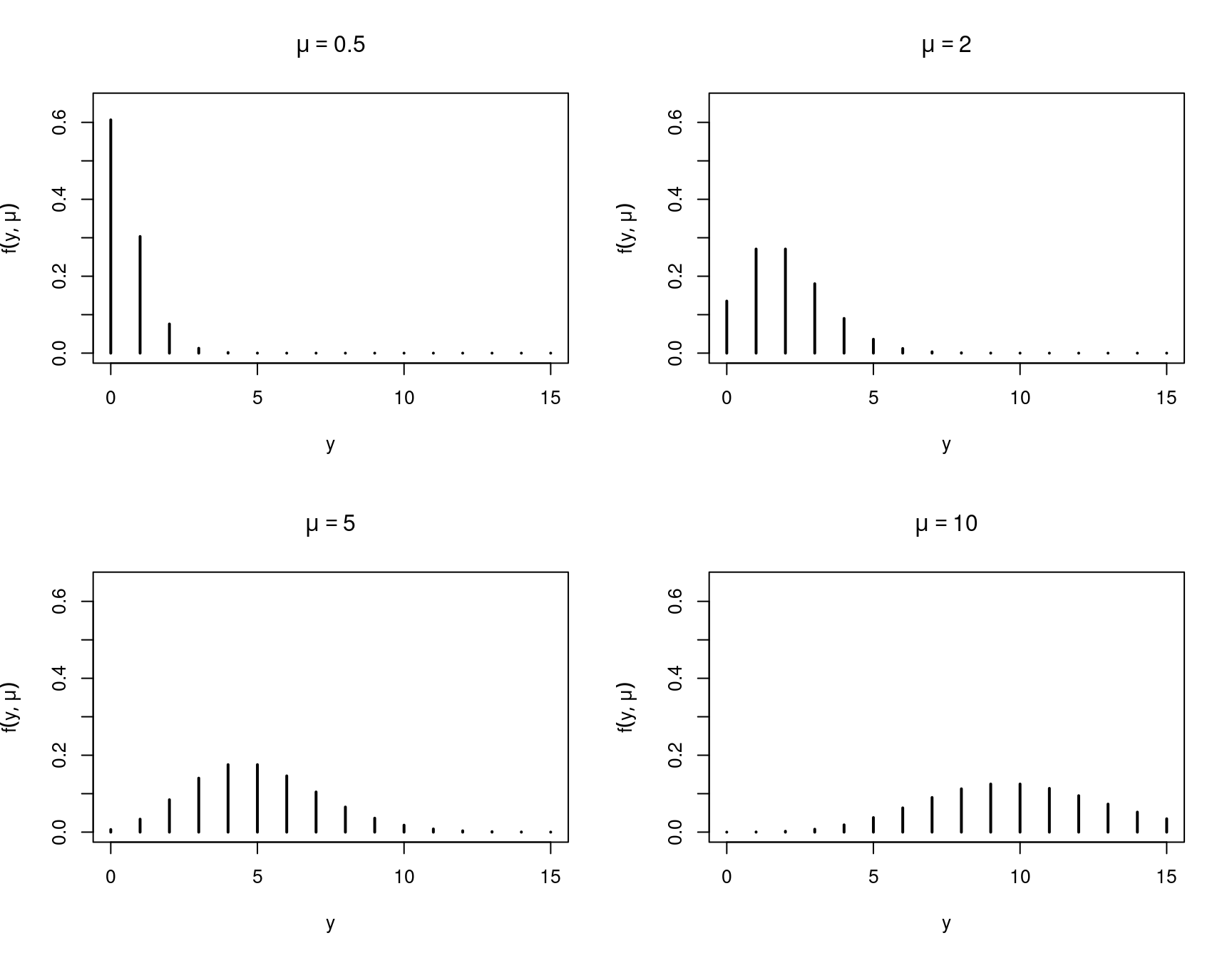

Figure 7.11: Poisson probability distribution with different means

While the PDF of the negative binomial distribution with the same \(\mu\) and \(\theta=10\) looks the following:

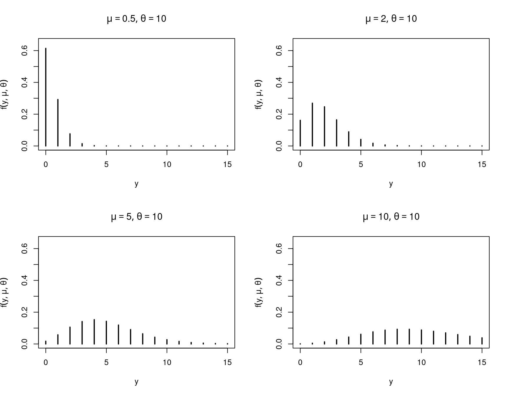
Figure 7.12: Negative binomial PDF with different means, theta=10

Regression: To employ the NB distribution in a regression, the natural mean equation is employed:

\[\begin{equation*} \log(\mu_i) ~=~ x_i^\top \beta. \end{equation*}\]

Variance: For the variance two different specifications are commonly used.

• NB2: Assume constant \(\alpha = 1/\theta\) and thus \(\text{Var}(y_i ~|~ x_i) = \mu_i + \alpha \cdot \mu_i^2\).
• NB1: Assume varying \(\theta_i\) such that \(\alpha = \mu_i / \theta_i\) and thus \(\text{Var}(y_i ~|~ x_i) = (1 + \alpha) \cdot \mu_i\).

NB1 and NB2 coincide without regressors but lead to differing models with regressors.

Note: For known \(\theta\) (e.g., \(\theta = 1\)), the negative binomial distribution belongs to an exponential family and thus falls into the GLM framework. For unknown \(\theta\) it is an extension.

In R: Package MASS provides negative.binomial(theta) family that can be plugged into glm(). glm.nb() is the extension that also estimates theta.

library("MASS")
rd_nb <- glm.nb(trips ~ ., data = RecreationDemand)
summary(rd_nb)

## 
## Call:
## glm.nb(formula = trips ~ ., data = RecreationDemand, init.theta = 0.7292568331, 
##     link = log)
## 
## Coefficients:
##             Estimate Std. Error z value Pr(>|z|)
## (Intercept) -1.12194    0.21430   -5.24  1.6e-07
## quality      0.72200    0.04012   18.00  < 2e-16
## skiyes       0.61214    0.15030    4.07  4.6e-05
## income      -0.02606    0.04245   -0.61    0.539
## userfeeyes   0.66917    0.35302    1.90    0.058
## costC        0.04801    0.00918    5.23  1.7e-07
## costS       -0.09269    0.00665  -13.93  < 2e-16
## costH        0.03884    0.00775    5.01  5.4e-07
## 
## (Dispersion parameter for Negative Binomial(0.7293) family taken to be 1)
## 
##     Null deviance: 1244.61  on 658  degrees of freedom
## Residual deviance:  425.42  on 651  degrees of freedom
## AIC: 1669
## 
## Number of Fisher Scoring iterations: 1
## 
## 
##               Theta:  0.7293 
##           Std. Err.:  0.0747 
## 
##  2 x log-likelihood:  -1651.1150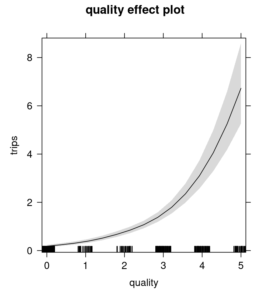

plot(Effect("quality", rd_nb), rescale.axis = FALSE)

Figure 7.13: Quality effect plot - negative binomial model

plot(Effect("income", rd_nb), rescale.axis = FALSE)

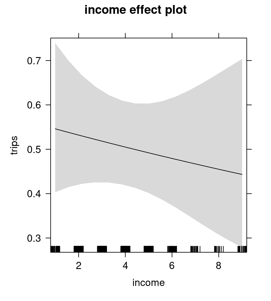
Figure 7.14: Income effect plot - negative binomial model

rootogram(rd_nb, max = 18)

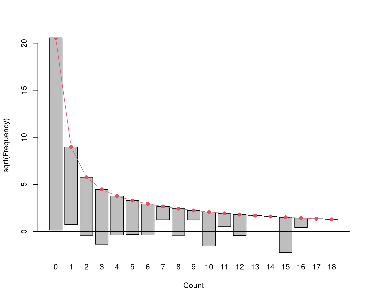
Figure 7.15: Hanging rootogram - negative binomial model

Likelihood ratio test: Test for overdispersion by comparing log-likelihoods of Poisson and NB2 model.

lrtest(rd_pois, rd_nb)

## Likelihood ratio test
## 
## Model 1: trips ~ quality + ski + income + userfee + costC + costS + costH
## Model 2: trips ~ quality + ski + income + userfee + costC + costS + costH
##   #Df LogLik Df Chisq Pr(>Chisq)
## 1   8  -1529                    
## 2   9   -826  1  1408     <2e-16

Note: The \(p\)-value is not valid, though. Standard ML theory does not apply because \(\theta = \infty\) (or \(\alpha = 0\)) is on the border of the parameter space. Here, the \(p\)-value has to be halved.

7.4.6 Unobserved heterogeneity

Furthermore: Other mixtures based on Poisson models \(h(y; \mu)\).

Continuous: Employ probability density function \(w(\mu)\) for

\[\begin{equation*} f(y) ~=~ \int_0^\infty h(y; \mu) ~ w(\mu) ~ d \mu. \end{equation*}\]

Using gamma, inverse normal, or lognormal distribution for \(w(\cdot)\) leads to negative binomial, PIG, or Poisson-lognormal distribution.

Finite: Employ weights \(w_j\) with \(\sum_{j = 1}^m w_j = 1\) for

\[\begin{equation*} f(y) ~=~ \sum_{j = 1}^m w_j \cdot h(y; \mu_j). \end{equation*}\]

7.5 Censoring and Truncation

Common problem: In microeconometrics, data are often incomplete or only partially observable.

Previously: Unobserved heterogeneity can be interpreted as lack of observability of explanatory variables.

Now: Limited data observability for dependent variables, e.g.,

• Truncation: Some observations omitted entirely from sample.
• Censoring: Some observations only known to be in limited range.

Truncation:

• Example: Asking unemployed workers about the number of unemployment spells, yields at least one unemployment spell.
• Typical case: Left-truncation at zero.
• Probability density function: For \(y_i > 0\)

\[\begin{equation*} f(y_i ~|~ y_i > 0, x_i) ~=~ \frac{f(y_i ~|~ x_i)}{1 ~-~ f(y_i = 0 ~|~ x_i)}. \end{equation*}\]

Censoring:

• Example: Survey with answer category ``more than \(a\)” (e.g., patents per year).
• Here: Right-censoring at \(a\) in original variable \(y_i^*\).
• Observation mechanism:

\[\begin{equation*} c_i ~=~ \left\{ \begin{array}{ll} 1 & \mbox{for } y_i^* \in A ~:=~ \{0, \dots, a\},\\ 0 & \mbox{for } y_i^* \in A' ~=~ \{a+1, a+2, \dots\}. \end{array} \right. \end{equation*}\]

• Thus: Observe \(y_i = y_i^*\) for \(c_i = 1\). Otherwise, exploit information that \(y_i^* > a\).
• Probability density function: Given \(c_i\)

\[\begin{equation*} \text{P}(Y_i ~=~ y_i ~|~ x_i)^{c_i} ~ \text{P}(Y_i ~>~ a ~|~ x_i)^{1 - c_i} ~=~ f(y_i ~|~ x_i)^{c_i} ~ \{1 - F(a ~|~ x_i)\}^{1 - c_i}. \end{equation*}\]

7.6 Hurdle and Zero-Inflated Count Data Models

7.6.1 Hurdle count data models

Idea: Account for excess (or lack of) zeros by two-part model.

• Is \(y_i\) equal to zero or positive? “Is the hurdle crossed?”
• If \(y_i > 0\), how large is \(y_i\)?

Formally:

• Zero hurdle: \(f_\text{zero}(y; z, \gamma)\). Binary part given by count distribution right-censored at \(y = 1\) (or simply Bernoulli variable).
• Count part: \(f_\text{count}(y; x, \beta)\). Count part given by count distribution left-truncated at \(y = 1\).

Combined: Probability density function for hurdle model,

\[\begin{eqnarray*} {f_\text{hurdle}(y; x, z, \beta, \gamma) } \\% && = \left\{ \begin{array}{ll} f_\text{zero}(0; z, \gamma), & y = 0, \\% \{ 1 - f_\text{zero}(0; z, \gamma) \} \cdot f_\text{count}(y; x, \beta)/\{1 - f_\text{count}(0; x, \beta)\}, & y > 0 . \end{array} \right. \end{eqnarray*}\]

Conditional mean: Using a log-link for the count component yields

\[\begin{equation*} \log(\mu_i) ~=~ x_i^\top \beta ~+~ \log(1 - f_\text{zero}(0; z_i, \gamma)) ~-~ \log(1 - f_\text{count}(0; x_i, \beta)). \end{equation*}\]

Warning: Literature has different parametrizations for \(f_\text{zero}\): Logit, probit, or censored count distribution. However, logit and censored geometric distribution coincide.

Example: Likelihood for Poisson hurdle model has two parts,

\[\begin{eqnarray*} \ell_1(\gamma) & = & \sum_{i: y_i = 0} \log H(z_i^\top \gamma) ~+~ \sum_{i: y_i > 0} \log \{ 1 - H(z_i^\top \gamma) \} \\ \ell_2(\beta) & = & \sum_{i: y_i > 0} \left[ \log f(y_i; \exp(x_i^\top \beta)) ~-~ \log \{ 1 - f(0; \exp(x_i^\top \beta)) \} \right]. \end{eqnarray*}\]

Remarks:

• Joint likelihood is \(\ell(\beta, \gamma) = \ell_1(\gamma) + \ell_2(\beta)\).
• Both parts can be maximized separately.
• Just requires software for binary response models and truncated count response models.

In R: hurdle() in pscl.

Formula: Two-part formula y ~ x1 + x2 | z1 + z2 + z3. Also, y ~ x1 + x2 is short for y ~ x1 + x2 | x1 + x2.

Distributions:

• dist specifies \(f_\text{count}\): "poisson" (default), "negbin" or "geometric".
• zero.dist specifies \(f_\text{zero}\): "binomial" (default, with varying links) or "poisson"/"negbin"/"geometric".

Hurdle test: If \(x = z\) and both components employ same count model, a test for the presence of the hurdle corresponds to \(H_0: \beta = \gamma\). In R: hurdletest().

rd_hp0 <- hurdle(trips ~ ., data = RecreationDemand,
  dist = "poisson", zero = "poisson")
summary(rd_hp0)

## 
## Call:
## hurdle(formula = trips ~ ., data = RecreationDemand, dist = "poisson", 
##     zero.dist = "poisson")
## 
## Pearson residuals:
##    Min     1Q Median     3Q    Max 
## -6.407 -0.357 -0.219 -0.169 13.331 
## 
## Count model coefficients (truncated poisson with log link):
##             Estimate Std. Error z value Pr(>|z|)
## (Intercept)  2.15040    0.11178   19.24  < 2e-16
## quality      0.04426    0.02385    1.86    0.063
## skiyes       0.46702    0.05879    7.94  2.0e-15
## income      -0.09770    0.02057   -4.75  2.1e-06
## userfeeyes   0.60069    0.07952    7.55  4.2e-14
## costC        0.00141    0.00396    0.36    0.722
## costS       -0.03661    0.00204  -17.92  < 2e-16
## costH        0.02388    0.00347    6.89  5.6e-12
## Zero hurdle model coefficients (censored poisson with log link):
##             Estimate Std. Error z value Pr(>|z|)
## (Intercept) -2.49906    0.27785   -8.99  < 2e-16
## quality      0.84848    0.05261   16.13  < 2e-16
## skiyes       0.44090    0.18443    2.39  0.01682
## income       0.00381    0.05039    0.08  0.93974
## userfeeyes   3.57526   73.99944    0.05  0.96147
## costC        0.00722    0.01700    0.42  0.67115
## costS       -0.05582    0.00920   -6.07  1.3e-09
## costH        0.04827    0.01329    3.63  0.00028
## 
## Number of iterations in BFGS optimization: 50 
## Log-likelihood: -1.18e+03 on 16 Df

hurdletest(rd_hp0)

## Wald test for hurdle models
## 
## Restrictions:
## count_((Intercept) - zero_(Intercept) = 0
## count_quality - zero_quality = 0
## count_skiyes - zero_skiyes = 0
## count_income - zero_income = 0
## count_userfeeyes - zero_userfeeyes = 0
## count_costC - zero_costC = 0
## count_costS - zero_costS = 0
## count_costH - zero_costH = 0
## 
## Model 1: restricted model
## Model 2: trips ~ .
## 
##   Res.Df Df Chisq Pr(>Chisq)
## 1    651                    
## 2    643  8   449     <2e-16

rd_hp <- hurdle(trips ~ . | quality + income,
  data = RecreationDemand, dist = "poisson")
rd_hnb <- hurdle(trips ~ . | quality + income,
  data = RecreationDemand, dist = "negbin")
modelsummary(list("Negbin hurdle"=rd_hnb, 
                  "Poisson hurdle" = rd_hp), 
             fmt=3, estimate="{estimate}{stars}")

	Negbin hurdle	Poisson hurdle
count_(Intercept)	0.842*	2.150***
	(0.383)	(0.112)
count_quality	0.172*	0.044+
	(0.072)	(0.024)
count_skiyes	0.622**	0.467***
	(0.190)	(0.059)
count_income	-0.057	-0.098***
	(0.065)	(0.021)
count_userfeeyes	0.576	0.601***
	(0.385)	(0.080)
count_costC	0.057**	0.001
	(0.022)	(0.004)
count_costS	-0.078***	-0.037***
	(0.012)	(0.002)
count_costH	0.012	0.024***
	(0.015)	(0.003)
zero_(Intercept)	-2.766***	-2.766***
	(0.362)	(0.362)
zero_quality	1.503***	1.503***
	(0.100)	(0.100)
zero_income	-0.045	-0.045
	(0.079)	(0.079)
Num.Obs.	659	659
R2	0.998	0.848
R2 Adj.	0.998	0.846
AIC	1554.2	2398.7
BIC	1608.1	2448.1
RMSE	23.38	5.35

7.6.2 Zero-inflated count data models

Different idea: Account for excess zeros via additional zero probability \(\pi = f_\text{zero}(0; z, \gamma)\).

Formally: Mixture model with two components.

\[\begin{eqnarray*} {f_\text{zeroinfl}(y; x, z, \beta, \gamma) } \\% && = f_\text{zero}(0; z, \gamma) \cdot I_{\{0\}}(y) ~+~ (1 - f_\text{zero}(0; z, \gamma)) \cdot f_\text{count}(y; x, \beta). \end{eqnarray*}\]

Conditional mean: Based on binomial GLM for unobserved probability for zero point mass

\[\begin{eqnarray*} \mu_i & = & \pi_i \cdot 0 ~+~ (1 - \pi_i) \cdot \exp(x_i^\top \beta), \\ \pi_i & = & g^{-1}(z_i^\top \gamma). \end{eqnarray*}\]

Remarks:

• Zeros have two sources: (1) Zero for sure in point mass. (2) Zero by chance in count component.
• Special cases: Zero-inflated Poisson (ZIP), zero-inflated negative binomial (ZINB).
• Likelihood cannot be separated as for hurdle models.
• ML estimation can be performed using EM (expectation-maximization) algorithm.

In R: zeroinfl() from package pscl with analogous interface to hurdle().

rd_zip <- zeroinfl(trips ~ . | quality + income,
  data = RecreationDemand, dist = "poisson")
rd_zinb <- zeroinfl(trips ~ . | quality + income,
  data = RecreationDemand, dist = "negbin")
modelsummary(list("Zero inflated negbin"=rd_zinb, 
                  "Zero inflated Poisson" = rd_zip), 
             fmt=3, estimate="{estimate}{stars}")

	Zero inflated negbin	Zero inflated Poisson
count_(Intercept)	1.097***	2.099***
	(0.257)	(0.111)
count_quality	0.169**	0.034
	(0.053)	(0.024)
count_skiyes	0.501***	0.472***
	(0.134)	(0.058)
count_income	-0.069	-0.100***
	(0.044)	(0.021)
count_userfeeyes	0.543+	0.610***
	(0.283)	(0.079)
count_costC	0.040**	0.002
	(0.015)	(0.004)
count_costS	-0.066***	-0.038***
	(0.008)	(0.002)
count_costH	0.021*	0.025***
	(0.010)	(0.003)
zero_(Intercept)	5.743***	3.292***
	(1.556)	(0.516)
zero_quality	-8.307*	-1.914***
	(3.682)	(0.206)
zero_income	-0.258	-0.045
	(0.282)	(0.108)
Num.Obs.	659	659
R2	0.986	0.851
R2 Adj.	0.986	0.849
AIC	1467.9	2383.6
BIC	1521.8	2433.0
RMSE	14.87	5.33

AIC(rd_hp, rd_hnb, rd_zip, rd_zinb, k = log(nrow(RecreationDemand)))

##         df  AIC
## rd_hp   11 2448
## rd_hnb  12 1608
## rd_zip  11 2433
## rd_zinb 12 1522

round(c(
  "Observed" = sum(RecreationDemand$trips < 1),
  "Poisson" = sum(dpois(0, fitted(rd_pois))),
  "NB" = sum(dnbinom(0, mu = fitted(rd_nb), size = rd_nb$theta)),
  "Hurdle-NB"= sum(predict(rd_hnb, type = "prob")[,1]),
  "ZINB" = sum(predict(rd_zinb, type = "prob")[,1])
))

##  Observed   Poisson        NB Hurdle-NB      ZINB 
##       417       277       423       417       433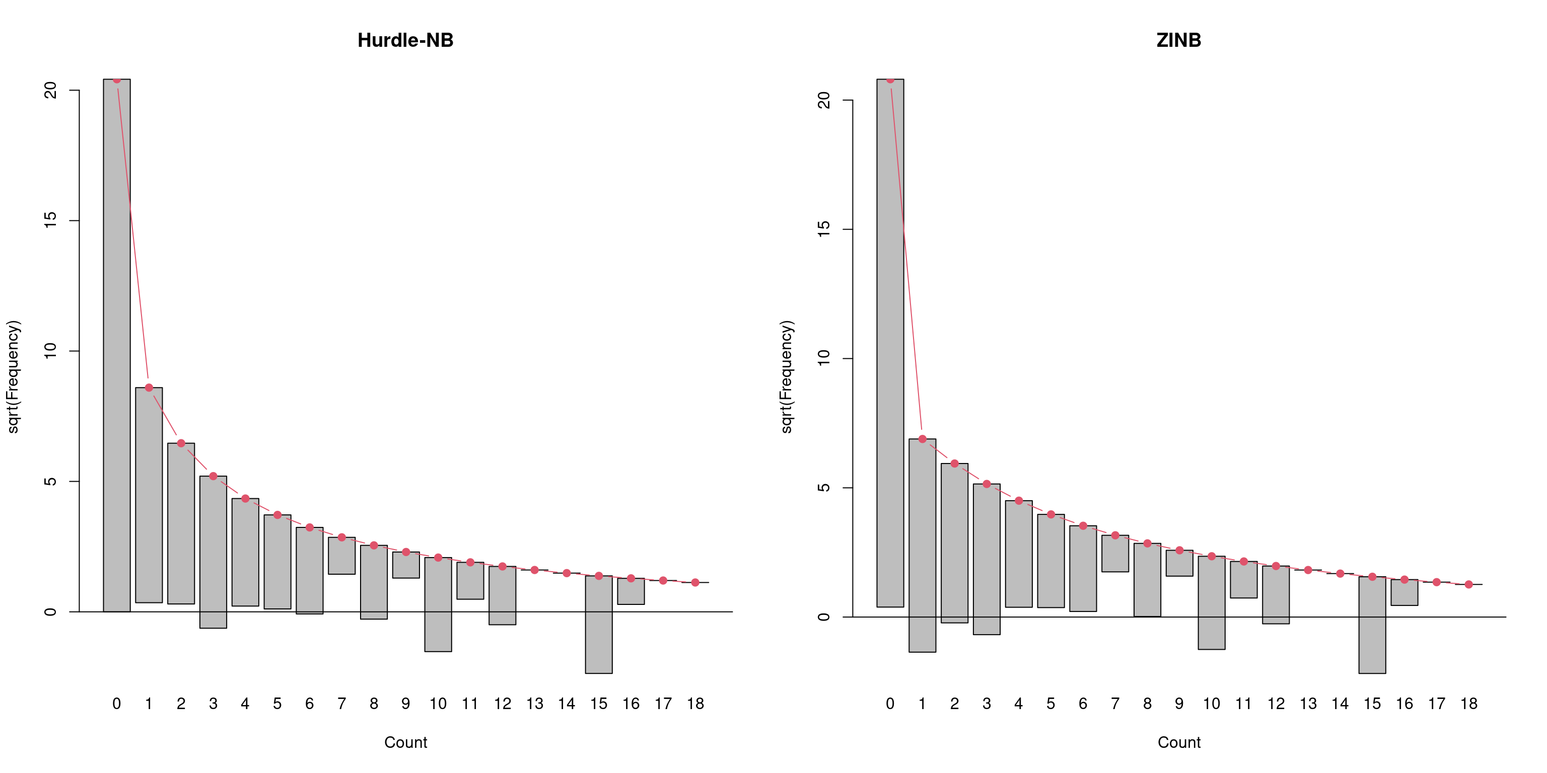

rootogram(rd_hnb, main = "Hurdle-NB", max = 18)
rootogram(rd_zinb, main = "ZINB", max = 18)

Figure 7.16: Hanging rootogram: Hurdle and zero inflated negative binomial model

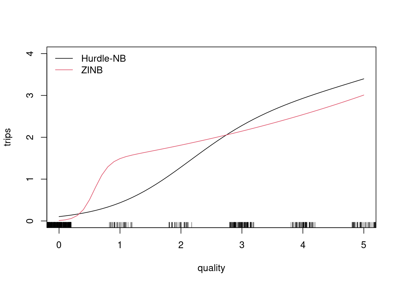
Figure 7.17: Effect of quality on trips: Hurdle and negative binomial model

7.7 Finite Mixture Count Data Models

Idea: Population is a mixture of \(m\) different populations and for each a (simple) parametric (regression) model holds. Membership for the \(m\) different “clusters” or “classes” is unknown in advance.

Formally: For prior weights/probabilities \(\omega_j \ge 0\) with \(\sum_{j = 1}^m \omega_j = 1\),

\[\begin{equation*} h(y_i; x_i, \omega_1, \dots, \omega_{m-1}, \beta_1, \dots, \beta_m) ~=~ \sum_{j = 1}^m \omega_j \cdot f(y_i; x_i, \beta_j), \end{equation*}\]

with \(f(y_i; \beta_j)\) being some parametric model, e.g., a Poisson or negative binomial regression for count data. The full parameter vector \(\theta = (\omega_1, \dots, \omega_{m-1}, \beta_1, \dots, \beta_m)\) has \((m-1) + m \cdot k\) parameters.

Interpretation: Clustering based on model, i.e., attractive for separating groups (such as healthy/ill individuals).

Terminology: Varies with community and basis model \(f(\cdot)\), e.g., finite mixture models, model-based clustering, latent class regression, cluster-wise regression, GLIMMIX.

Problems:

• No generally accepted criterion/heuristic for choosing \(m\).
• The latent weights \(\omega_j\) are only defined up to permutation. Sometimes ordering is induced by requiring \(\omega_1 \le \omega_2 \le \dots \le \omega_m\).
• Estimation would be easy if “hard” cluster/class memberships were known (corresponding to models of type y ~ class * x in R).

Task: Need to optimize full log-likelihood

\[\begin{equation*} \ell(\theta) ~=~ \sum_{i = 1}^n \log h(y_i; x_i, \theta) ~=~ \sum_{i = 1}^n \log \left( \sum_{j = 1}^m \omega_j \cdot f(y_i; x_i, \beta_j) \right). \end{equation*}\]

Solution: Typically achieved using expectation-maximization (EM) algorithm, a general strategy for optimizing complex likelihoods with latent variables.

E step: Expectation of posterior class probabilities \(w_{ij}\)

\[\begin{eqnarray*} \hat w_{ij} & = & \text{P}(j ~|~ y_i, x_i, \hat \theta) ~=~ \frac{\hat \omega_j \cdot f(y_i; x_i, \hat \beta_j)}{\sum_{k = 1}^m \hat \omega_k \cdot f(y_i; x_i, \hat \beta_k)} \\ \hat \omega_j & = & \frac{1}{n} \sum_{i = 1}^n \hat w_{ij}. \end{eqnarray*}\]

M step: Maximization of log-likelihood in each component

\[\begin{equation*} \hat \beta_j ~=~ \underset{\beta_j}{argmax} \sum_{i = 1}^n \hat w_{ij} \cdot \log f(y_i; x_i, \beta_j). \end{equation*}\]

Iterate until convergence.

In R:

• Package flexmix provides flexible mixture model framework.
• Package provides E step, leverages available model fitting functions for M step.
• Note that M step corresponds to fitting model y ~ x with weights = w_j(\(w_{1j}, \dots, w_{nj}\)).
• Alternatively, “hard” (instead of “soft”) classification can be used by setting weights to 0 or 1 (for class \(j\) with highest weight).
• New drivers providing M~steps can be plugged into package flexmix.

Example: Try to separate “high” users from “low” users in RecreationDemanddata.

library("flexmix")
set.seed(4002)
rd_fm <- flexmix(trips ~ ., data = RecreationDemand, k = 2,
  model = FLXMRglm(trips ~ ., family = "poisson"))
summary(rd_fm)

## 
## Call:
## flexmix(formula = trips ~ ., data = RecreationDemand, k = 2, 
##     model = FLXMRglm(trips ~ ., family = "poisson"))
## 
##        prior size post>0 ratio
## Comp.1  0.81  589    640 0.920
## Comp.2  0.19   70    606 0.116
## 
## 'log Lik.' -949.9 (df=17)
## AIC: 1934   BIC: 2010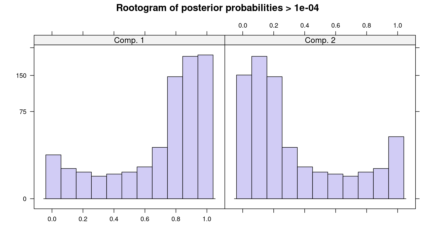

plot(rd_fm)

Figure 7.18: Rootogram of posterior probabilities

summary(refit(rd_fm))

## $Comp.1
##             Estimate Std. Error z value Pr(>|z|)
## (Intercept) -1.87856    0.25400   -7.40  1.4e-13
## quality      0.79767    0.04712   16.93  < 2e-16
## skiyes       0.23247    0.13995    1.66  0.09669
## income      -0.01074    0.04259   -0.25  0.80088
## userfeeyes   1.21230    0.26737    4.53  5.8e-06
## costC       -0.03888    0.01108   -3.51  0.00045
## costS       -0.01446    0.00367   -3.94  8.0e-05
## costH        0.05146    0.00990    5.20  2.0e-07
## 
## $Comp.2
##             Estimate Std. Error z value Pr(>|z|)
## (Intercept)   1.9311     0.3403    5.67  1.4e-08
## quality      -0.1178     0.0525   -2.24  0.02491
## skiyes        1.3298     0.1799    7.39  1.4e-13
## income        0.0115     0.0497    0.23  0.81737
## userfeeyes   -0.5547     0.1682   -3.30  0.00097
## costC         0.0813     0.0112    7.23  4.8e-13
## costS        -0.1612     0.0191   -8.44  < 2e-16
## costH         0.0531     0.0119    4.48  7.5e-06

7.8 Summary and Outlook

7.8.1 Summary

Available strategies:

• Basic model: Poisson. Often too restrictive as conditional probability model (in microeconomic applications).
• Conditional mean model: Keep mean equation, give up remaining likelihood, employ robust standard errors.
• Overdispersion: Negative binomial (as conditional probability model) or quasi-Poisson (as conditional mean model).
• Excess zeros: Hurdle model or zero-inflation model (based on Poisson or negative binomial).
• Unobserved clusters: Finite mixture models.

7.8.2 Outlook

Further methods:

• Models without zeros: zero-truncation models. (In R: package countreg on R-Forge.)
• Alternative continuous mixtures: Poisson-lognormal, PIG, etc.
• Generalizations of negative binomial distribution: NegBin-\(P\), NegBin-H (multiple index model with conditional dispersion parameter).
• Other generalized count distributions, e.g., generalized Poisson etc.
• Multivariate count response models.
• Other semiparametric models, …