Chapter 4 Binary Response Models
4.1 Introduction
In this chapter we examine binary response models, in which the dependent variable can only take up values zero and one. Typical economic examples of binary variables include:
- Labor market participation of women.
\(y_i\): Woman \(i\) works/does not work.
Potential covariates: Age, education, children, … - Who is member of the workers’ union?
\(y_i\): Person \(i\) is/is not member of the workers’ union.
Potential covariates: Age, education, occupation, … - Default of consumer credits, credit scoring.
\(y_i\): Person \(i\) pays/does not pay credit back.
Potential covariates: Income, credit history, maturity, occupation, age, marital status, … - Choice of mode of transportation.
\(y_i\): Person \(i\) uses/does not use public transport to travel to work.
Potential covariates: Distance, costs, …
Microeconomic theory often assumes continuous choice within convex budget sets. However, in practice many choices are necessarily discrete, e.g., the purchase of a car. Furthermore, even continuous, ordered, or multinomial variables are sometimes transformed to binary variables. For example, a binary variable happy/unhappy could be derived from happiness on a scale 0–10, where a score up to 5 is assigned the value “unhappy”, and a score above 5 counts as “happy”. In such situations we lose information, however, this simplification often provides a good first answer due to its simple specification and its ease of interpretation.
4.2 GLMs for Binary Response Variables
As \(y_i \in \{0, 1\}\), the only conceivable model is the Bernoulli probability function with
\[\begin{equation*} f(y_i ~|~ x_i) ~=~ \pi_i^{y_i} ~ (1 - \pi_i)^{1 - y_i}, \end{equation*}\]
where \(\pi_i = \text{Prob}(y_i = 1 ~|~ x_i)\), the conditional probability of observing an outcome of one. Hence, conditional mean and conditional variance are:
\[\begin{eqnarray*} \text{E} (y_i ~|~ x_i) & = & \pi_i,\\ \text{Var}(y_i ~|~ x_i) & = & \pi_i ~ (1 - \pi_i). \end{eqnarray*}\]
For parameterization, typically the GLM approach is employed, i.e., \(g(\pi_i) ~=~ x_i^\top \beta\), where \(g: [0, 1] \rightarrow \mathbb{R}\) is the link function.
4.2.1 Link functions
As derived in Chapter 2, the canonical link corresponds to the log-odds (or logits).
\[\begin{equation*} g(\pi) ~=~ \log \left( \frac{\pi}{1 - \pi} \right) ~=:~ \text{logit} (\pi_i). \end{equation*}\]
The regression model with this link is known as logit model (more common in econometrics) or logistic regression (more common in statistics) because
\[\begin{equation*} g^{-1}(\eta) ~=~ \frac{\exp(\eta)}{1 + \exp(\eta)} ~=~ \frac{1}{1 + \exp(-\eta)} ~=:~ \Lambda(\eta) \end{equation*}\]
is the cumulative distribution function (CDF) of the logistic distribution. Also, recall that the dispersion is \(\phi = 1\) and the variance function is \(\text{Var}(\pi) = \pi (1 - \pi)\). More generally, other cumulative distribution functions, denoted by \(H(\cdot)\) with \(H: \mathbb{R} \rightarrow [0, 1]\), i.e., other functions that map a real number onto the unit interval, can also be used as the inverse link function:
\[\begin{equation*} \pi_i ~=~ H(x_i^\top \beta) ~=~ H(\eta_i). \end{equation*}\]
Note that the associated probability density function (PDF) \(h(\cdot)\) then corresponds to \(\partial \pi / \partial \eta\), or, in generic GLM notation: \(\partial \mu / \partial \eta\). The most common alternative to logit models is the probit model, defined as \(g(\pi) = \Phi^{-1}(\pi)\). Here, \(H(\eta) = \Phi(\eta)\) is the standard normal cumulative distribution function. A further alternative is the complementary log-log link, defined as \(g(\pi) = \log(-\log(1 - \pi))\), where the corresponding \(H(\eta) = 1 - \exp(-\exp(\eta))\) is the CDF of a type of extreme-value or Gumbel distribution. Although the complementary log-log link is typically not used in econometrics, it is available in R, along with further links. To compare the most generally used logit vs. probit links, let’s examine their densities:
\[\begin{eqnarray*} \mbox{Logit: } h(\eta) & = & \frac{\exp(-\eta)}{(1 + \exp(-\eta))^2} \quad (=:~ \lambda(\eta)).\\ \mbox{Probit: } h(\eta) & = & \frac{1}{\sqrt{2 \pi}} \exp \left(- \frac{\eta^2}{2} \right) \quad (=:~ \phi(\eta)). \end{eqnarray*}\]
Note that both distributions are symmetric around zero. The standard deviation of a standard logistic distribution, however, is \(\pi/\sqrt{3} \approx 1.814\), i.e., not \(1\) as for the standard normal distribution. The slopes at \(\eta = 0\) are also different between the two links: for logit models it is \(\lambda(0) = 0.25\) while for probit models it is \(\phi(0) \approx 0.40\). Hence, the scaling differs by a factor of \(\phi(0)/\lambda(0) \approx 1.60\). The shape of the two distributions is very similar, but the logistic distribution has somewhat heavier tails, as illustrated in the following graph. Thus, if observations in the tails (i.e., close to 0 or 1) are avoided, logit and probit models are very similar. Keep in mind, however, that the scaling of the coefficients is different.
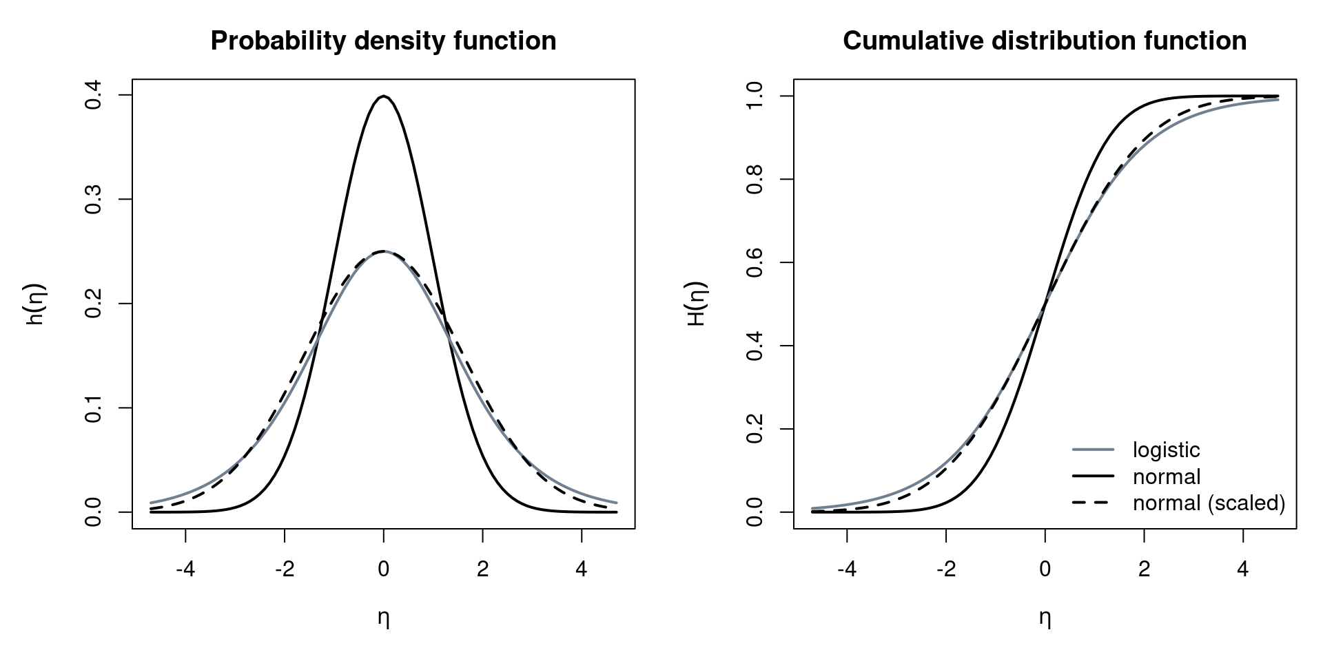
Figure 4.1: Visual Comparison of Normal and Logistic Distribution
A further motivation for using the probit model is the latent variable approach. Let \(y_i^*\) be a latent (i.e., unobservable) variable that captures the continuous propensity for a “success”, e.g., to work or to default, and is subject to some error \(\varepsilon_i\). If the latent variable exceeds some threshold zero, without loss of generality, a success is observed, i.e.,
\[\begin{eqnarray*} y_i^* & = & x_i^\top \beta ~+~ \varepsilon_i \\ y_i & = & I(y_i^* \ge 0) ~=~ \left\{ \begin{array}{ll} 1 & \mbox{if} \\ 0 & \mbox{if not} \end{array} \right. y_i^* \ge 0. \end{eqnarray*}\]
Thus, if \(H(\cdot)\) is the CDF of the negative error \(-\varepsilon_i\):
\[\begin{eqnarray*} \pi_i & = & \text{Prob} (y_i^* \ge 0 ~|~ x_i) ~=~ \text{Prob}(x_i^\top \beta + \varepsilon_i \ge 0 ~|~ x_i) \\ & = & \text{Prob} (\varepsilon_i \ge - x_i^\top \beta ~|~ x_i) ~=~ \text{Prob}(- \varepsilon_i \le x_i^\top \beta ~|~ x_i) \\ & = & H(x_i^\top \beta). \end{eqnarray*}\]
In probit models, if the negative error term is normally distributed with variance \(\sigma^2\) and mean \(\mu\) (to reflect a different threshold than zero),
\[\begin{equation*} \pi_i ~=~ \text{Prob} (- \varepsilon_i \le x_i^\top \beta ~|~ x_i) ~=~ \Phi \left( \frac{x_i^\top \beta - \mu}{\sigma} \right) ~=~ \Phi (x_i^\top \tilde \beta) \end{equation*}\]
where \(\tilde \beta = ((\beta_1 - \mu)/\sigma, \beta_2/\sigma, \dots, \beta_k/\sigma)^\top\). Notice that the probability depends on both \(\beta\) and \(\sigma\), so that the two individual parameters cannot be identified. As only the ratio \(\beta/\sigma\) is identified, if both \(\beta\) and \(\sigma\) are scaled by the same constant, their ratio, and thus the probability of success, is unchanged. This results in indefinitely many parameter pairs that lead to the same outcome. We call this overparameterization. The solution to overparameterization is to normalize some of the parameters. If, for example, only the difference \(\beta_1 - \mu\) identified, we can set the latent mean to zero (\(\mu = 0\)). In the case of binary response models, only the ratio \(\beta_j/\sigma\) is identified, and thus we typically fix the scaling of the latent variable \(\sigma = 1\), so that the parameters are uniquely defined.
Analogously, the logit link can be viewed as a latent variable with logistic errors, or alternatively, as a linear model on a log-odds scale, i.e., taking exponential transforms to an odds scale. Odds are defined as
\[\begin{equation*} \text{odds}(\mathit{event}) ~=~ \frac{\text{Prob}(\mathit{event})}{1 - \text{Prob} (\mathit{event})}. \end{equation*}\]
Therefore, odds can be computed as
\[\begin{equation*} \frac{\text{Prob}(y_i = 1 ~|~ x_i)}{\text{Prob}(y_i = 0 ~|~ x_i)} ~=~ \frac{\pi_i}{1 - \pi_i} ~=~ \exp(x_i^\top \beta). \end{equation*}\]
Two (groups of) subjects can be easily compared by so-called odds ratios:
\[\begin{eqnarray*} \frac{\text{odds}(y_a = 1 ~|~ x_a)}{\text{odds}(y_b = 1 ~|~ x_b)} & = & \frac{\exp(x_a^\top \beta)}{\exp(x_b^\top \beta)} \\ & = & \exp(x_a^\top \beta - x_b^\top \beta) \\ & = & \exp((x_a - x_b)^\top \beta) \end{eqnarray*}\]
As an example, consider two subjects \(x_a\) and \(x_b\) where \(x_a = x_b + \Delta x_{bl}\) differ only for the \(l\)-th regressor by one unit \(\Delta x_{bl} = (0, \dots, 1, \dots, 0)^\top\). Then, the odds ratio above simplifies to \(\exp(\beta_l)\), and the relative change in the odds ratio is \(\exp(\beta_l) - 1\). Note that for “small” \(\beta_l\) , \(\exp(\beta_l) - 1 \approx \beta_l\), i.e., small coefficients can be interpreted directly as relative changes in odds ratios.
4.2.2 Interpretation of parameters
In the previous section, we have seen that the exp of a coefficient \(\exp(\beta_l)\) for \(l>1\) in a logit model can be interpreted as relative changes in the odds of “success” for a 1-unit increase in a certain regressor \(x_l\), ceteris paribus. There are two problems with this way of interpretation: Firstly, it only works for models with a logit link. For probit models, there is no such ceteris paribus interpretation available. Secondly, the interpretation is in terms of odds, rather than probabilities, which most practitioners find easier to interpret.
The intercept \(\beta_1\) is interpreted in logit models by taking its inverse link transformation \(\Lambda(\beta_1)\), and interpret it as the probability of “success” for the case where all \(x_j=0\) for \(j>0\). This interpretation of the intercept works analogously in probit models, with \(\Phi(\cdot)\) as the inverse link transformation. Notice that this only pertains to one specific combination of regressors, which may, or may not be realistic. For example, the regressor age is unlikely to take up zero as a value in data sets concerning adults.
The following graphics illustrate the different effects the intercept \(\beta_1\) and a single slope coefficient \(\beta_2\) have on probability, depending on \(x\).
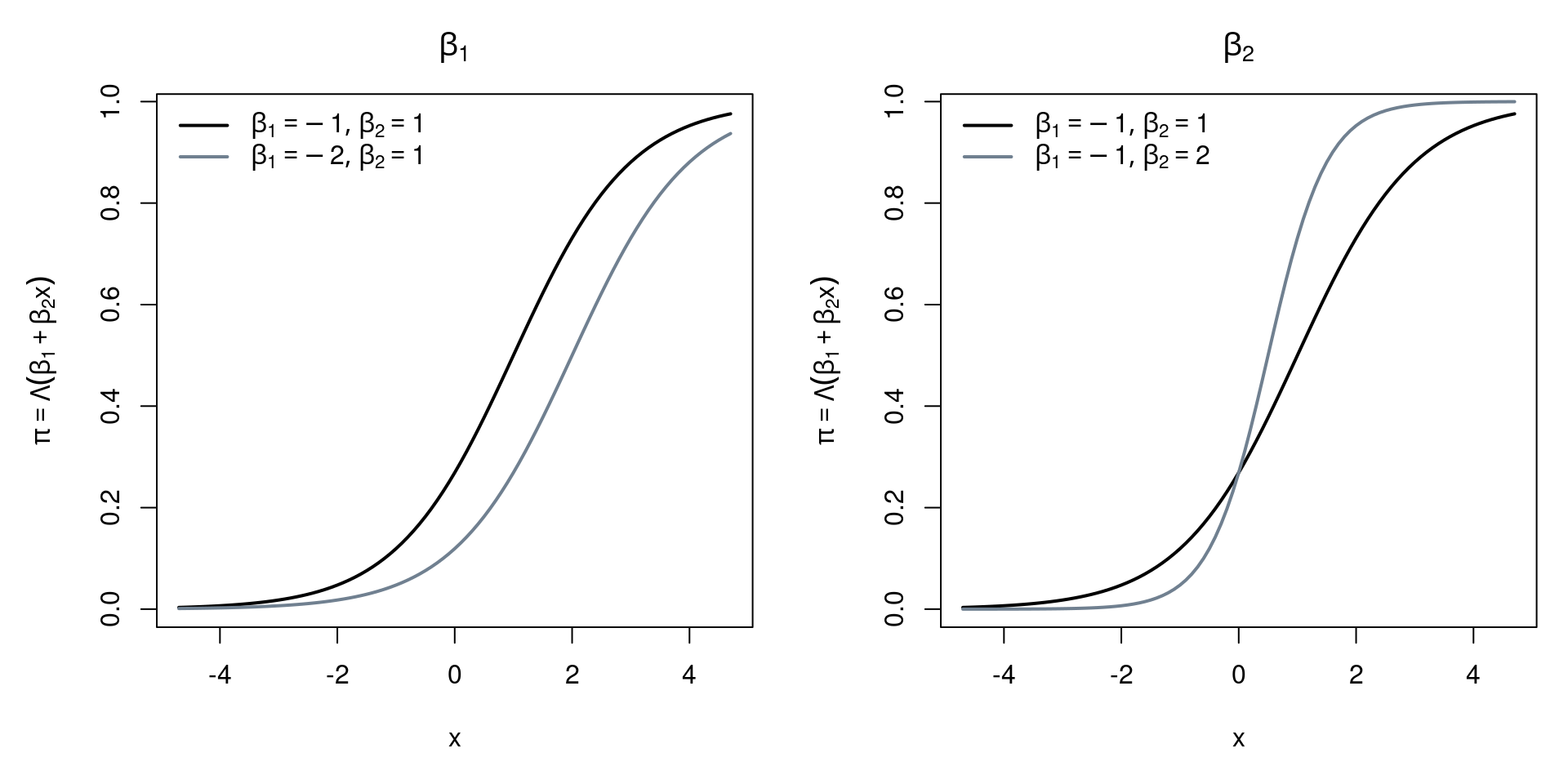
Figure 4.2: Effects of Coefficients on Probability
We know that in the linear regression model, parameters \(\beta_j\) capture the expected changes in the response variable.
\[\begin{equation*} \frac{\partial \text{E} (y_i ~|~ x_i)}{\partial x_{il}} ~=~ \frac{\partial (x_i^\top \beta)}{\partial x_{il}} ~=~ \beta_l. \end{equation*}\]
In the binomial GLM, however, the partial derivatives, and thus the marginal effects, are not constant:
\[\begin{equation*} \frac{\partial \text{E}(y_i ~|~ x_i)}{\partial x_{il}} ~=~ \frac{\partial H(x_i^\top \beta)}{\partial x_{il}} ~=~ h(x_i^\top \beta) \cdot \beta_l. \end{equation*}\]
Some important properties of MPE are:
- The sign of the marginal effect is equal to the sign of \(\beta_l\)
- The effect is largest for \(x_i^\top \beta = 0\) for symmetric unimodal \(h(\cdot)\)
- The effect varies among individuals
In practice, we usually report “typical” effects by taking expectations. This can be done two ways: we either estimate expected marginal probability effect (MPE) \(\text{E}_x(h(x_i^\top \beta)) \beta_l\) by average MPE (AMPE) \(1/n \sum_{i = 1}^n h(x_i^\top \beta) \beta_l\), or we estimate MPE at expected regressor \(h(E(x)^\top \beta) \beta_l\) by MPE at mean regressor \(h(\bar x^\top \beta) \beta_l\). Remember that taking means can be plausible for continuous regressors but it is hard to interpret for categorical regressors, and thus also for dummy variables pertaining to those. A better solution is to evaluate MPE in different groups (e.g., foreign and Swiss, men and women), or, alternatively, to assess the influence graphically by plotting \(\text{E}(y ~|~ x)\) against \(x_l\), while keeping all except \(l\)-th regressor at a typical value such as \(\bar x_{-l}\). In other words, we examine the marginal effect of one chosen regressor, while fixing all other regressors at their mean. Keep in mind that all previous computations assume that there is a one-to-one relationship between variables and regressors \(x_{il}\). This is violated when variables occur in multiple regressors, e.g., in interactions or polynomials. For example, in case of a quadratic polynomial \(\text{E} (y ~|~ x) = H(\beta_1 + \beta_2 x + \beta_3 x^2)\):
\[\begin{equation*} \frac{\partial \text{E} (y ~|~ x)}{\partial x} ~=~ h(\beta_1 + \beta_2 x + \beta_3 x^2) \cdot (\beta_2 + 2 \beta_3 x). \end{equation*}\]
This is typically ignored in software packages that offer automatic computation of marginal effects. In R, we can employ the margins package which correctly deals with polynomials.
4.2.3 Example: Swiss labor participation
In this section, we are going to analyze cross-section data on Swiss labor participation, originating from the health survey SOMIPOPS for Switzerland in 1981 (Gerfin 1996). The data frame contains 872 observations on the following 7 variables:
| Variable | Description |
|---|---|
participation |
Factor. Did the individual participate in the labor force? |
income |
Logarithm of nonlabor income. |
age |
Age in decades (years divided by 10). |
education |
Years of formal education. |
youngkids |
Number of young children (under 7 years). |
oldkids |
Number of older children (over 7 years). |
foreign |
Factor. Is the individual a foreigner? |
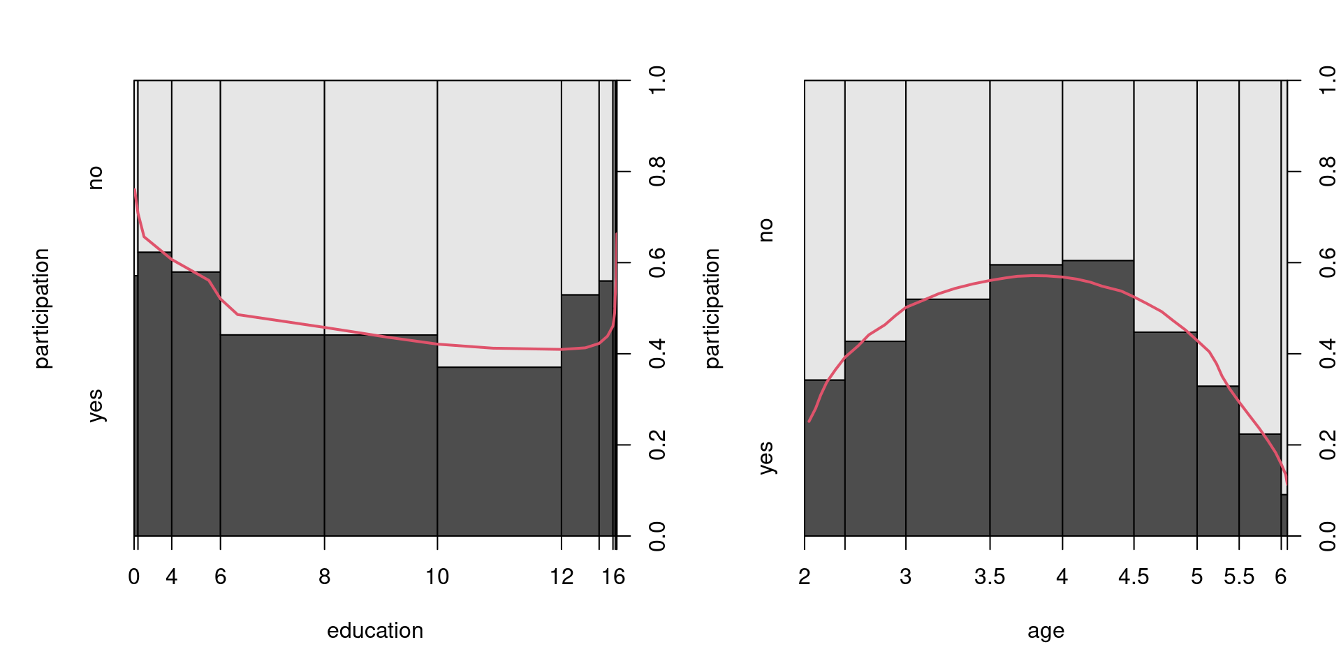
Figure 4.3: Labor Participation Depending on Age and Education
- Estimation: First, we fit a logit model with all explanatory variables (
~ .in R), and a quadratic polynomial in age.
data("SwissLabor", package = "AER")
swiss_logit <- glm(participation ~ . + I(age^2),
  data = SwissLabor, family = binomial)
summary(swiss_logit)
##
## Call:
## glm(formula = participation ~ . + I(age^2), family = binomial,
## data = SwissLabor)
##
## Coefficients:
## Estimate Std. Error z value Pr(>|z|)
## (Intercept) 6.1964 2.3831 2.60 0.0093
## income -1.1041 0.2257 -4.89 1.0e-06
## age 3.4366 0.6879 5.00 5.9e-07
## education 0.0327 0.0300 1.09 0.2761
## youngkids -1.1857 0.1720 -6.89 5.5e-12
## oldkids -0.2409 0.0845 -2.85 0.0043
## foreignyes 1.1683 0.2038 5.73 9.9e-09
## I(age^2) -0.4876 0.0852 -5.72 1.0e-08
##
## (Dispersion parameter for binomial family taken to be 1)
##
## Null deviance: 1203.2 on 871 degrees of freedom
## Residual deviance: 1017.6 on 864 degrees of freedom
## AIC: 1034
##
## Number of Fisher Scoring iterations: 4- Prediction: Then, we compute predictions of the response variable \(\hat \pi_i\). (The default is prediction of linear predictor \(\hat \eta_i\).)
predict(swiss_logit, data.frame(income = 11, age = 3.3,
  education = 12, youngkids = 1, oldkids = 1, foreign = "no"),
  type = "response")
## 1
## 0.2783predict(swiss_logit, data.frame(income = 11, age = 3.3,
education = 12, youngkids = 1, oldkids = 1, foreign = "yes"),
type = "response")## 1
## 0.5536- Odds ratios: Compute the ratio of odds for working between foreign and Swiss women, first, without standardizing for other regressors. One way to do this is to compute an empirical contingency table, the associated proportions, odds, and odds ratio. A second way to compute odds ratios is by fitting a binomial GLM with logit link and take exp of the estimated coefficient for the foreign indicator variable, leading to the same result:
##        participation
## foreign  no yes
##     no  402 254
## yes 69 147## participation
## foreign no yes
## no 0.6128 0.3872
## yes 0.3194 0.6806## no yes
## 0.6318 2.1304## yes
## 3.372##
## Call: glm(formula = participation ~ foreign, family = binomial, data = SwissLabor)
##
## Coefficients:
## (Intercept) foreignyes
## -0.459 1.215
##
## Degrees of Freedom: 871 Total (i.e. Null); 870 Residual
## Null Deviance: 1200
## Residual Deviance: 1150 AIC: 1150## foreignyes
## 3.372We can also compute odds ratios for a marginal one unit change in all variables (ceteris paribus).
##     income  education  youngkids    oldkids foreignyes
##     0.3315     1.0332     0.3055     0.7859     3.2167
As mentioned earlier, we need to be careful with polynomials because the assumption of a one-to-one relationship between the variable and the regressors is violated as the variable occurs in multiple regressors. In this model, for example, due to the age polynomial, the odds ratio depends on age itself. Consider a one-year change in age for a 30- and 50-year old woman.
##   age
## 1.047## age
## 0.8617We can thus use the margins package to calculate expected marginal probability effects (MPE).:
##      factor     AME     SE       z      p   lower   upper
##         age -0.0820 0.0167 -4.9099 0.0000 -0.1148 -0.0493
##   education  0.0065 0.0060  1.0917 0.2750 -0.0052  0.0182
##  foreignyes  0.2431 0.0407  5.9774 0.0000  0.1634  0.3228
##      income -0.2204 0.0428 -5.1435 0.0000 -0.3044 -0.1364
##     oldkids -0.0481 0.0166 -2.9017 0.0037 -0.0806 -0.0156
## youngkids -0.2367 0.0309 -7.6719 0.0000 -0.2972 -0.1762- Effects: To assess our findings graphically, we visualize the change in probability for a partial (one unit) change in one regressor, given typical values for all other regressors. To make R understand that
ageand|I(age^2)|should be treated as a single term, usepoly(age, 2, raw = TRUE)instead of adding the latter as an additional regressor.
swiss_logit2 <- glm(participation ~ income + education +
  poly(age, 2, raw = TRUE) + youngkids + oldkids + foreign,
  data = SwissLabor, family = binomial)
Visualization using the effects package:
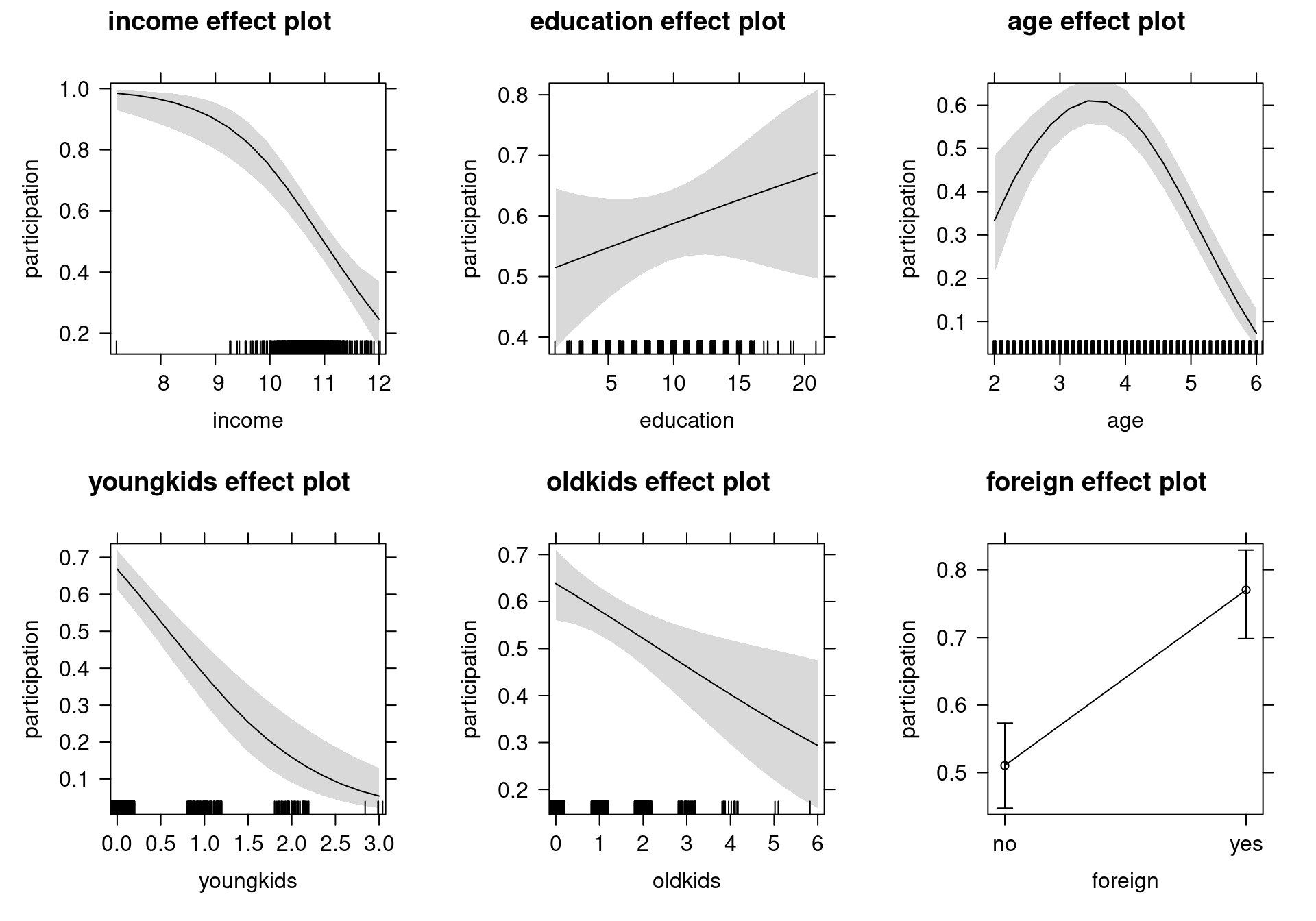
Figure 4.4: Effects of Explanatory Variables on Labor Force Participation - Logit Model
- Inference: Next we can test whether a quadratic polynomial in education significantly improves the model:
- Wald test:
swiss_logit3 <- glm(participation ~ . + I(age^2) + I(education^2),
  data = SwissLabor, family = binomial)
coeftest(swiss_logit3)[9,]
## Estimate Std. Error z value Pr(>|z|)
## 0.009812 0.006002 1.634796 0.102092## Wald test
##
## Model 1: participation ~ income + age + education + youngkids + oldkids +
## foreign + I(age^2)
## Model 2: participation ~ income + age + education + youngkids + oldkids +
## foreign + I(age^2) + I(education^2)
## Res.Df Df Chisq Pr(>Chisq)
## 1 864
## 2 863 1 2.67 0.1- Likelihood ratio test (via analysis of deviance):
## Analysis of Deviance Table
##
## Model 1: participation ~ income + age + education + youngkids + oldkids +
##     foreign + I(age^2)
## Model 2: participation ~ income + age + education + youngkids + oldkids +
##     foreign + I(age^2) + I(education^2)
##   Resid. Df Resid. Dev Df Deviance Pr(>Chi)
## 1       864       1018
## 2 863 1015 1 2.65 0.1- Likelihood ratio test (via generic lmtest approach):
## Likelihood ratio test
##
## Model 1: participation ~ income + age + education + youngkids + oldkids +
##     foreign + I(age^2)
## Model 2: participation ~ income + age + education + youngkids + oldkids +
##     foreign + I(age^2) + I(education^2)
##   #Df LogLik Df Chisq Pr(>Chisq)
## 1   8   -509
## 2 9 -507 1 2.65 0.1- The probit model: Probit estimation leads to virtually identical results.
swiss_probit <- glm(participation ~ income + education +
  poly(age, 2, raw = TRUE) + youngkids + oldkids + foreign,
  data = SwissLabor, family = binomial(link = "probit"))
modelsummary(list("Logit model"= swiss_logit2, "Probit model" = swiss_probit),
fmt=3, estimate="{estimate}{stars}")| Logit model | Probit model | |
|---|---|---|
| (Intercept) | 6.196** | 3.749** |
| (2.383) | (1.407) | |
| income | -1.104*** | -0.667*** |
| (0.226) | (0.132) | |
| education | 0.033 | 0.019 |
| (0.030) | (0.018) | |
| poly(age, 2, raw = TRUE)1 | 3.437*** | 2.075*** |
| (0.688) | (0.405) | |
| poly(age, 2, raw = TRUE)2 | -0.488*** | -0.294*** |
| (0.085) | (0.050) | |
| youngkids | -1.186*** | -0.714*** |
| (0.172) | (0.100) | |
| oldkids | -0.241** | -0.147** |
| (0.084) | (0.051) | |
| foreignyes | 1.168*** | 0.714*** |
| (0.204) | (0.121) | |
| Num.Obs. | 872 | 872 |
| AIC | 1033.6 | 1033.2 |
| BIC | 1071.7 | 1071.3 |
| Log.Lik. | -508.785 | -508.577 |
| F | 20.055 | 22.819 |
| RMSE | 0.45 | 0.45 |
##               (Intercept)                    income                 education
##                     1.653                     1.655                     1.702
## poly(age, 2, raw = TRUE)1 poly(age, 2, raw = TRUE)2                 youngkids
##                     1.656                     1.657                     1.660
##                   oldkids                foreignyes
## 1.639 1.635## [1] 1.596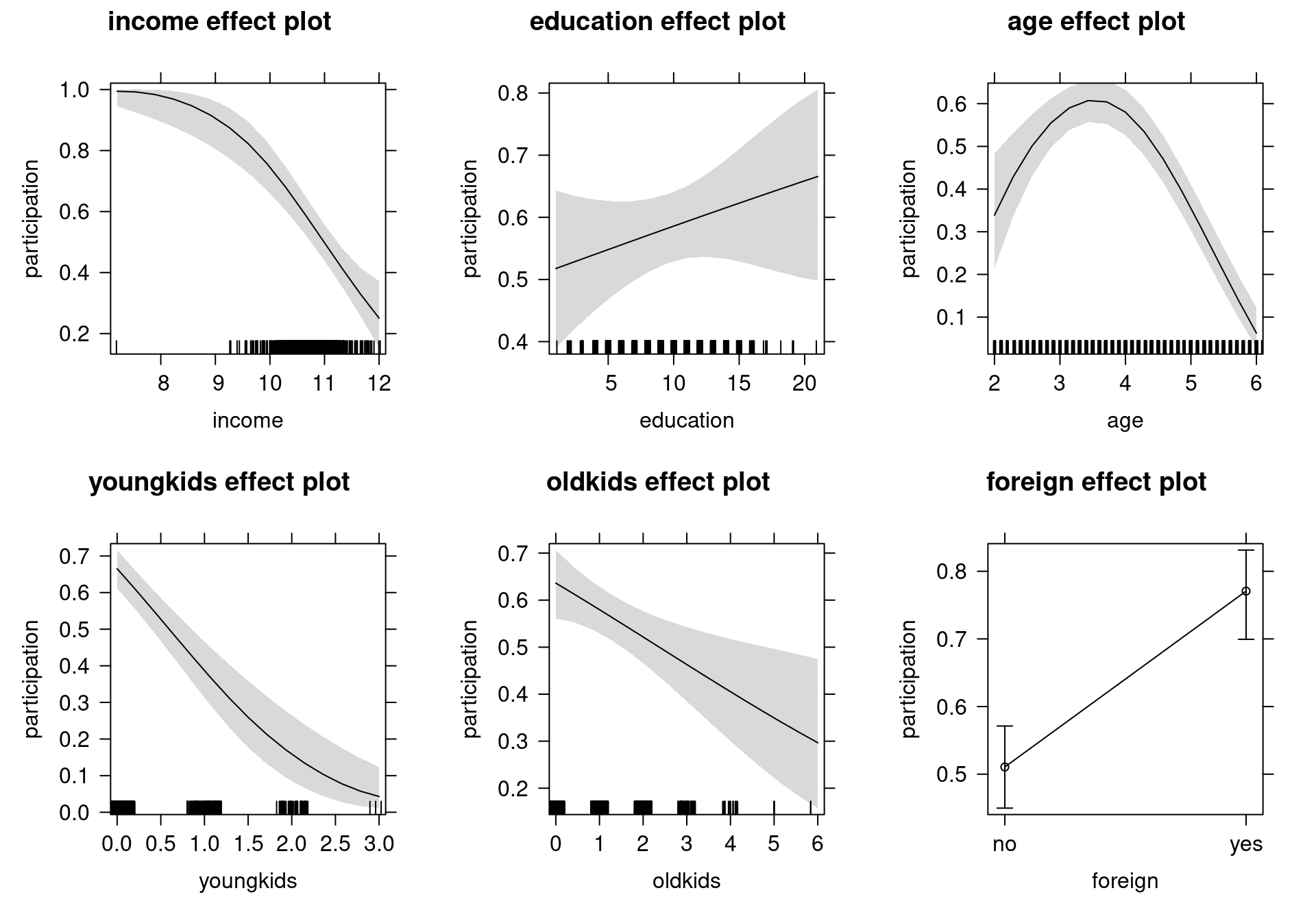
Figure 4.5: Effects of Explanatory Variables on Labor Force Participation - Probit Model
4.2.4 The linear probability model
Instead of using binary GLMs, many practitioners prefer running linear regressions using OLS on a 0/1-coded response. This is also known as the linear probability model. The main advantage is that coefficients can be directly interpreted as marginal changes in the success probabilities without having to consider any relative changes in odds or other nonlinear transformations.
However, this advantage does not come for free. It is clear that OLS cannot be an efficient estimator because binary observations (i.e., from a Bernoulli distribution) are necessarily heteroscedastic and the variance changes along with the mean: \(Var(y_i ~|~ x_i) = \pi_i \cdot (1 - \pi_i)\). But practitioners argue that even under heteroscedasticity, the OLS estimator is consistent, and that inference can easily be adjusted by using “robust” sandwich standard errors.
This consistency is only obtained, though, under the assumption that the mean equation \(E(y_i ~|~ x_i) = \pi_i = x_i^\top \beta\) is correctly specified. As the success probability is bounded \(\pi_i \in [0, 1]\) while the linear predictor \(x_i^\top \beta\) is not, this assumption cannot hold in general. Moreover, as the variance is a direct transformation of the expectation in binary regressions for cross-section data, it is not possible to correctly specify the latter and potentially misspecify the former. Thus, if the variance is misspecified, the expectation is also, and OLS is inconsistent. Conversely, if the expectation is correctly specified, the variance is known as well and it is not necessary to employ “robust” sandwich standard errors.
Thus, from a theoretical perspective it is hard to justify the linear probability model. However, a more pragmatic take is that the linearity assumption for the expectation may actually work well enough in practice, at least if the fitted probabilities avoid the extremes of \(0\) and \(1\) sufficiently clearly. In such cases, the marginal effects from a binary GLM are typically approximately constant and roughly equal to the coefficients from the linear probability model.
As an example, see the following fitting of a linear model to the Swiss labor participation data. Notice that both conditional mean and variance are misspecified in this model.
SL2 <- SwissLabor
SL2$participation <- as.numeric(SL2$participation) - 1
swiss_lpm <- lm(participation ~ . + I(age^2), data = SL2)
coeftest(swiss_lpm, vcov=sandwich)
##
## t test of coefficients:
##
## Estimate Std. Error t value Pr(>|t|)
## (Intercept) 1.66368 0.39725 4.19 3.1e-05
## income -0.21284 0.03554 -5.99 3.1e-09
## age 0.68254 0.11997 5.69 1.7e-08
## education 0.00666 0.00579 1.15 0.2504
## youngkids -0.24063 0.03007 -8.00 3.9e-15
## oldkids -0.04931 0.01743 -2.83 0.0048
## foreignyes 0.24960 0.04017 6.21 8.1e-10
## I(age^2) -0.09703 0.01452 -6.68 4.2e-11## Min. 1st Qu. Median Mean 3rd Qu. Max.
## 0.0104 0.2806 0.4703 0.4607 0.6183 0.9416## Min. 1st Qu. Median Mean 3rd Qu. Max.
## -0.255 0.308 0.475 0.460 0.601 1.027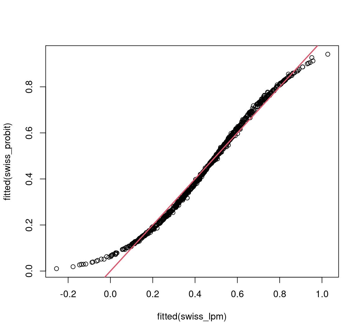
Figure 4.6: Linear vs. Probit model fitted values
modelsummary(list("Linear model"=swiss_lpm, "Probit model"=swiss_probit),
vcov=sandwich, fmt=3, estimate="{estimate}{stars}")| Linear model | Probit model | |
|---|---|---|
| (Intercept) | 1.664*** | 3.749** |
| (0.397) | (1.327) | |
| income | -0.213*** | -0.667*** |
| (0.036) | (0.127) | |
| age | 0.683*** | |
| (0.120) | ||
| education | 0.007 | 0.019 |
| (0.006) | (0.018) | |
| youngkids | -0.241*** | -0.714*** |
| (0.030) | (0.106) | |
| oldkids | -0.049** | -0.147** |
| (0.017) | (0.052) | |
| foreignyes | 0.250*** | 0.714*** |
| (0.040) | (0.122) | |
| I(age^2) | -0.097*** | |
| (0.015) | ||
| poly(age, 2, raw = TRUE)1 | 2.075*** | |
| (0.399) | ||
| poly(age, 2, raw = TRUE)2 | -0.294*** | |
| (0.050) | ||
| Num.Obs. | 872 | 872 |
| R2 | 0.193 | |
| R2 Adj. | 0.186 | |
| AIC | 1091.3 | 1033.2 |
| BIC | 1134.2 | 1071.3 |
| Log.Lik. | -536.647 | -508.577 |
| RMSE | 0.45 | 0.45 |
| Std.Errors | Custom | Custom |
4.3 Discrete Choice Models
Discrete choice models based on random utility maximization provide a further - economic - motivation for using binary models. They connect binary response models with microeconomic models of choice based on utility maximization problems subject to constraints. Consider the choice between two alternatives \(A\) and \(B\) (e.g., products/brands) with alternative-specific attributes \(z_{i, A}\) and \(z_{i, B}\) (e.g., price) and individual-specific characteristics \(x_i\) (e.g., age). The linear utility function with random error terms (also called random utility) is:
\[\begin{eqnarray*} u_{i, A} & = & x_i^\top \beta_A ~+~ z_{i, A}^\top \gamma ~+~ \varepsilon_{i, A}, \\ u_{i, B} & = & x_i^\top \beta_B ~+~ z_{i, B}^\top \gamma ~+~ \varepsilon_{i, B}. \end{eqnarray*}\]
Person \(i\) chooses alternative \(A\) (“success”: \(y_i = 1\)) if the corresponding utility is larger \(u_{i, A} > u_{i, B}\). Thus, the probability for choosing \(A\) is
\[\begin{eqnarray*} & = & \text{Prob} (u_{i, A} > u_{i, B} ~|~ x_i, z_{i, A}, z_{i, B}) \\ & = & \text{Prob} (x_i^\top (\beta_A - \beta_B) + (z_{i, A} - z_{i, B})^\top \gamma + (\varepsilon_{i, A} - \varepsilon_{i, B}) ~\ge~ 0 ~|~ x_i, z_{i, A}, z_{i, B}) \\ & = & \text{Prob} (- \varepsilon_i ~\le~ x_i^\top \beta ~+~ z_i^\top \gamma ~|~ x_i, z_i) \\ & = & \text{Prob} (- \varepsilon_i ~\le~ {x^*_i}^\top \beta^* ~|~ x^*_i) \\ & = & H({x^*_i}^\top \beta^*), \end{eqnarray*}\]
if we write \(\beta = \beta_A - \beta_B\), \(z = z_A - z_B\), \(\varepsilon = \varepsilon_A - \varepsilon_B\), and \(\beta^* = (\beta_A - \beta_B, \gamma)\), \(x^*_i = (x_i, z_{i, A} - z_{i, B})\). Notice that only the difference between the coefficients of the two alternatives \(\beta = \beta_A - \beta_B\) is identified. Moreover, alternative-specific parameters \(\gamma\) can only be estimated if attributes \(z_{i, A} - z_{i, B}\) vary across individuals \(i\).
The intercept in this case reflects whether ceteris paribus option \(A\) or \(B\) is more attractive. Moreover, if utility is normally distributed, i.e., if \(\varepsilon_A\) and \(\varepsilon_B\) are normally distributed, the difference in errors \(\varepsilon\) is also normal, which leads to the probit model. However, if the random component of the utility is assumed to have a type-I extreme value or Gumbel distribution, the difference \(\varepsilon\) has a logistic distribution, thus leading to the logit model. Due to their motivation, these models are also called random utility models (RUMs).
4.4 Goodness of Fit
Measuring the Goodness of Fit is more controversial in binary data than in numeric, and there are two main ideas for its assessment. One is to use a similar measure as \(R^2\) in linear regression, i.e., to create a measure that indicates goodness of fit in the unit interval. One problem with measuring the goodness of fit in terms of \(R^2\), even in numeric data, is that it is always problematic to asses what counts as a satisfactory \(R^2\) for a given model. Macroeconomic models, where most input quantities are strongly aggregated, have typically much higher \(R^2\) than it is possible to achieve for individual choice models, for example. Nevertheless, in a linear regression, an \(R^2\) has a clear meaning and interpretation as a variance decomposition. This is not the case for binary models, thus we call these Pseudo \(R^2\). A pseudo \(R^2\) measures the goodness of fit of a binary model in the unit interval, where 0 indicates a complete lack of fit, and 1 corresponds to a perfect fit. However, these measures are typically not proportionate within the unit interval, thus they are difficult to interpret. We first examine some of the most used options for pseudo \(R^2\) measures.
The McFadden \(R^2\) is constructed the following way: As \(\ell(\beta) \le 0\), one can exploit that \(|\ell(\hat \beta)| \le |\ell(\bar \beta)|\) where \(\bar \beta\) is the fit from the intercept-only model.
\[\begin{equation*} 0 ~\le~ 1 - \frac{\ell(\hat \beta)}{\ell(\bar \beta)} ~=:~ R_{\text{McFadden}}^2 ~\le~ 1. \end{equation*}\]
This will only become \(1\) in the limit for a perfect prediction. Another pseudo \(R^2\) measure by McKelvey and Zavoina \(R^2\) employs the error sum of squares (\(\mathit{SSE}\)) and residual sum of squares (\(\mathit{RSS}\)) on a linear predictor scale.
\[\begin{eqnarray*} R_{\text{MZ}}^2 & = & \frac{\mathit{SSE}}{\mathit{SSR} + \mathit{SSE}}, \\ \mathit{SSE} & = & \sum_{i = 1}^n (\hat \eta_i - \bar{\hat{\eta}})^2, \\ \mathit{SSR} & = & n \sigma^2. \end{eqnarray*}\]
Where the variance \(\sigma^2\) is determined by the link function, i.e., \(\sigma^2 = 1\) for the probit and \(\sigma^2 = \pi^2/3\) for the logit. The Cox and Snell \(R^2\) uses the likelihood instead of the log-likelihood:
\[\begin{equation*} R_{\text{CS}}^2 ~=~ 1 - \left( \frac{L(\bar \beta)}{L(\hat \beta)} \right)^{2/n}. \end{equation*}\]
And lastly, the Nagelkerke/Cragg and Uhler \(R^2\) is a normalized version of \(R_{\text{CS}}^2\), because its maximum \(R_{\text{CS,max}}^2 = 1 - L(\bar \beta)^{2/n} \neq 1\).
\[\begin{equation*} R_{\text{N/CU}}^2 ~=~ R_{\text{CS}}^2 / R_{\text{CS,max}}^2. \end{equation*}\]
There are many more pseudo \(R^2\) existing for binary data, and there is no universally accepted, or even “best” \(R^2\) measure available.
The second possibility to measure the goodness of fit in binary models is to assess the model’s predictive performance, i.e., to assess in sample or out of sample predictions. To illustrate this, let’s compare logit and probit specification for Swiss labor data.:
## [1] 1018## [1] 1017## 'log Lik.' -508.8 (df=8)## 'log Lik.' -508.6 (df=8)swiss_logit0 <- update(swiss_logit, formula = . ~ 1)
1 - as.vector(logLik(swiss_logit)/logLik(swiss_logit0))## [1] 0.1543swiss_probit0 <- update(swiss_probit, formula = . ~ 1)
1 - as.vector(logLik(swiss_probit)/logLik(swiss_probit0))## [1] 0.1546We can see that both models appear to have virtually identical fits. We thus create a confusion matrix, which is a contingency table of observed vs. predicted values, by choosing some cutoff \(c\). A cutoff of \(c = 0.5\) would mean that under a probability of 0.5, a woman is predicted not to participate in the labor force, while for a probability over 0.5 she is predicted to do so. This yields correct predictions (main diagonal: true negatives and true positives) and incorrect predictions (off-diagonal: false negatives and false positives).
##      pred
## true  FALSE TRUE
##   no    337  134
## yes 146 255## pred
## true FALSE TRUE
## no 337 134
## yes 146 255It is then possible to consider all conceivable cutoffs \(c \in [0, 1]\) and compute various performance measures.
- Accuracy: \(\text{ACC}(c)\) is the proportion of correct predictions (among all observations).
- True positive rate: \(\text{TPR}(c)\) is the proportion of correct predictions (among observations with \(y_i = 1\)).
- False positive rate: \(\text{FPR}(c)\) is the proportion of incorrect predictions (among observations with \(y_i = 0\)).
- Receiver operator characteristic: \(\text{ROC} = \{ (\text{FPR}(c), \text{TPR}(c)) ~|~ c \in [0, 1] \}\). Ideally, this should be as close as possible to left upper corner \((0, 1)\).
- Area under the curve: Aggregate measure that summarizes the whole ROC curve is the associated area under the curve (AUC).
In R, all these measures can easily be computed and graphed using the ROCR package. First, set up an object with predicted and observed values:
Then compute and plot accuracy:
Compute and plot False positive rate vs. True positive rate, i.e., the ROC curve:
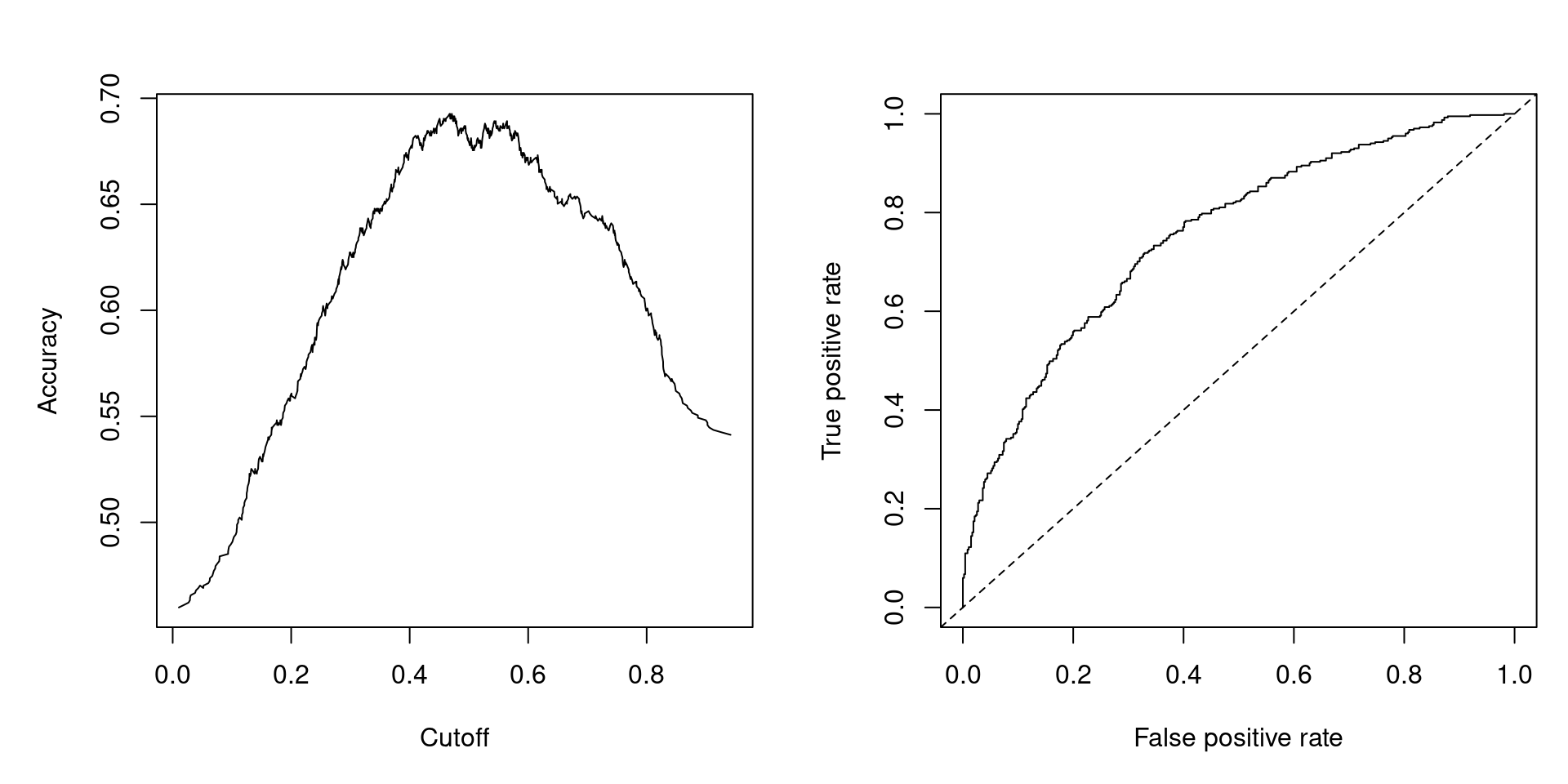
Figure 4.7: Accuracy at Different Cutoffs and ROC Curve
4.5 Perfect Prediction and (Quasi-)Complete Separation
(Log-)Likelihood is given by:
\[\begin{eqnarray*} L(\beta) & = & \prod_{i = 1}^n \pi_i^{y_i} ~ (1 - \pi_i)^{1 - y_i} ~=~ \prod_{i = 1}^n H(x_i^\top \beta)^{y_i} ~ (1 - H(x_i^\top \beta))^{1 - y_i} ~\le~ 1, \\ \ell(\beta) & = & \sum_{i = 1}^n \left\{ y_i ~ \log H(x_i^\top \beta) ~+~ (1 - y_i) ~ \log \{ 1 - H(x_i^\top \beta) \} \right\} ~\le~ 0. \end{eqnarray*}\]
The Likelihood function is “well-behaved”: it is bounded and can be shown to be globally concave for logit/probit. However, the maximum does not have to be assumed for finite \(\beta\). For example, let’s assume that there is a \(k+1\)-st regressor that is perfectly correlated with response, e.g., \(x_{i, k+1} = 0\) if \(y_i = 0\) and \(x_{i, k+1} = 1\) if \(y_i = 1\), i.e., the outcome \(y_i\) is \(0\) whenever the regressor is \(0\), and \(1\) whenever the regressor takes up \(1\) as a value. Using \(\tilde x_i = (x_i, x_{i, k+1})\) and \(\tilde \beta = (\beta, \beta_{k + 1})^\top\):
\[\begin{eqnarray*} \ell(\beta) & = & \sum_{i = 1}^n \left\{ y_i ~ \log H(\tilde x_i^\top \tilde \beta) ~+~ (1 - y_i) ~ \log \{ 1 - H(\tilde x_i^\top \tilde \beta) \} \right\} \\ & = & \sum_{x_{i, k+1} = 1} \log H(x_i^\top \beta ~+~ \beta_{k + 1}) \\ & & ~+~ \sum_{x_{i, k+1} = 0} \left\{ y_i ~ \log H(x_i^\top \beta) ~+~ (1 - y_i) ~ \log \{ 1 - H(x_i^\top \beta) \} \right\}. \end{eqnarray*}\]
While the second term could be maximized as usual, the first term is monotonically increasing in \(\beta_{k+1}\). Thus, for logit/probit, the maximum (\(= 0\)) is only attained in the limit for \(\beta_{k+1} \rightarrow \infty\). More generally, we say the data are quasi-completely separated if there is a \(\beta_0\) such that
\[\begin{eqnarray*} y_i ~=~ 0 \mbox{ if } x_i^\top \beta_0 ~\le~ 0, \\ y_i ~=~ 1 \mbox{ if } x_i^\top \beta_0 ~\ge~ 0. \\ \end{eqnarray*}\]
While they are completely separated if strict inequality holds. In words, complete separation occurs when one of the regressors is perfectly correlated with the outcome, while quasi-complete separation occurs when a regressor can predict at least one of the resulting classes perfectly.
There are two possible solutions to the problem of (quasi-) complete separation. The first option is to assess separated groups, if separation is believed to be structural rather than by chance. The second one is to employ some regularized estimator (i.e., with penalty on \(|\beta|\)). For an example of quasi complete separation, let’s examine a cross-section data set on executions in different states in 1950 (Maddala 2001, Table 8.4, p. 330), containing 44 observations on 8 variables.
| Variable | Description |
|---|---|
rate |
Murder rate per 100,000 (FBI estimate, 1950). |
convictions |
Number of convictions divided by murders in 1950. |
executions |
Average number of executions during 1946–1950 divided by convictions in 1950 |
time |
Median time served (in months) of convicted murderers released in 1951. |
income |
Median family income in 1949 (in 1,000 USD). |
lfp |
Labor force participation rate in 1950 (in percent). |
noncauc |
Proportion of non-Caucasian population in 1950. |
southern |
Factor indicating region. |
data("MurderRates", package = "AER")
murder_logit <- glm(I(executions > 0) ~ time + income + noncauc + lfp + southern,
                    data = MurderRates, family = binomial)
## Warning: glm.fit: fitted probabilities numerically 0 or 1 occurred##
## z test of coefficients:
##
## Estimate Std. Error z value Pr(>|z|)
## (Intercept) 10.9933 20.7734 0.53 0.597
## time 0.0194 0.0104 1.87 0.062
## income 10.6101 5.6541 1.88 0.061
## noncauc 70.9879 36.4118 1.95 0.051
## lfp -0.6676 0.4767 -1.40 0.161
## southernyes 17.3313 2872.1707 0.01 0.995Notice that the southern variable has a large coefficient and an extremely large standard error. For this reason, even though the variable is relevant, it is not meaningful to estimate coefficients and p-values (for the latter, non-standard inference would be needed).
murder_logit2 <- glm(I(executions > 0) ~ time + income + noncauc + lfp + southern,
                     data = MurderRates, family = binomial,
                     control = list(epsilon = 1e-15, maxit = 50, trace = FALSE))
## Warning: glm.fit: fitted probabilities numerically 0 or 1 occurredmodelsummary(
list("Default" = murder_logit, "More iterations" = murder_logit2),
fmt = 3, estimate = "{estimate}{stars}")| Default | More iterations | |
|---|---|---|
| (Intercept) | 10.993 | 10.993 |
| (20.773) | (2.077e+01) | |
| time | 0.019+ | 0.019+ |
| (0.010) | (1.000e-02) | |
| income | 10.610+ | 10.610+ |
| (5.654) | (5.654e+00) | |
| noncauc | 70.988+ | 70.988+ |
| (36.412) | (3.641e+01) | |
| lfp | -0.668 | -0.668 |
| (0.477) | (4.770e-01) | |
| southernyes | 17.331 | 31.331 |
| (2872.171) | (1.733e+07) | |
| Num.Obs. | 44 | 44 |
| AIC | 981.1 | 1282.3 |
| BIC | 991.8 | 1293.0 |
| Log.Lik. | -484.536 | -635.157 |
| F | 1.520 | |
| RMSE | 0.25 | 0.25 |
Comparing the two models, we can see that all coefficients and standard errors remain the same, except for the “southernyes” variable’s coefficient and standard error, which both diverge to infinity.
The problem becomes visible once we create a contingency table of executions > 0 vs. southern. In southern states, executions were always nonzero, which means the data is quasi-completely separated for the southern variable. Whenever the southern variable takes up “yes” as a value, it immediately implies that the number of executions in the given state is nonzero in the sample.
##
##         no yes
##   FALSE  9   0
##   TRUE  20  15
In practice, when standard errors are unusually large, one should locate the problem by changing the number of iterations, or drop some variables, etc. Be aware that some software packages - including the software Maddala used- do not report any error in this situation. Other software packages give verbose error messages. In R, this is available in safeBinaryRegression. Regularized estimators (instead of ML) are available in R in brglm (bias-reduced GLMs) or bayesglm in arm (Bayesian estimation).