Chapter 1 Introduction
1.1 What Is Microeconometrics?
The Econometric Society was founded on the 29th of December 1930 in Cleveland. Co-founder Ragnar Frisch described its purpose as “an international society for the advancement of economic theory in its relation to statistics and mathematics” in the first volume of Econometrica in 1933 (for more information see https://en.wikipedia.org/wiki/Econometrics). In 1969, the first Nobel Prize in Economics was awarded to Ragnar Frisch and Jan Tinbergen, followed by many subsequent Nobel Prizes for econometricians or economists with strong quantitative research. In 2000, two “microeconometricians” were awarded the prize: James J. Heckman “for his development of theory and methods for analyzing selective samples”, and Daniel McFadden “for his development of theory and methods for analyzing discrete choice”.
We differentiate between two types of empirical analysis: Theory-based empirical analysis starts with a microeconomic question as a motivation behind it, and is based on a formal economic model or theory. Then, quantities of interest are determined and testable hypotheses are derived based on the theory. One typical model would be individual decisions or behavior as a function of exogenous parameters. In other words, theory comes first, and the objective is to prove the theory.
It is often difficult, though, to have a fully developed economic model. In some cases, the underlying theories might not exist, or they might need modification. We call this theory-building empirical analysis. Theory-building empirical analysis is possible because the principles of empirical analysis of microdata are mostly independent of the underlying theory. For this type of analysis, a good grasp of data structures and associated empirical/statistical methods is required. In other words, empirical data comes first, from which a model is built, and the theory is further advanced based on the outcome.
1.2 What Are Microdata?
The three most important features of microdata:
- cross-sectional (focus of this course) or micropanels (which we will briefly touch)
- often have non-continuous measurement scale
- mostly observational (rarely experimental)
Examples for economic data in general include: cross-section data for 5,000 households for the year 2009, time series data for one country over 25 years, and panel data: 5,000 households over 5 years (“micropanel”), or 12 countries over 25 years (“macropanel”). Typically, microeconometrics deals with cross-sectional data and micropanels, while macroeconomics deals with time-series data and macropanels.
The two main categories of microdata are quantitative and qualitative. Quantitative microdata can be either discrete or continuous, and can have an unrestricted range, or a restricted range (e.g. counts, durations, censored, truncated). Qualitative microdata, also called categorical, has three main types: binary, multinomial and ordered. Models for microdata are typically determined by the type of the dependent variable.
1.2.1 Quantitative microdata
The default assumptions for a quantitative dependent variable are: (1) Its support is the real line. This is compatible with the assumption that the dependent variable is normally distributed, and conditional on regressors. (2) Observations form a random sample of the population, which excludes systematic discrepancy between the population and the selected sample. Both of these assumptions, however, are frequently violated in microdata applications. Some examples include:
Non-negative variables: wages of workers and house prices are non-negative and thus cannot be normally distributed, although in some cases the normal distribution can be an adequate approximation. A special case of non-negative variables is duration between events (e.g., duration of unemployment, time to relapse of criminals).
Frequent zeros: A continuous positive variable with a cluster of observations at zero, e.g., expenditures for (durable) consumer goods, like cars or refrigerators, over the last year. Zero then corresponds to a corner solution of a household utility maximization problem.
Truncated variables: We call a variable truncated if all observations above or below a certain threshold are excluded from the sample. An example of a truncated variable is the distribution of SAT (Standardized Aptitude Test) scores among admitted students, rather than among all applicants. The sample is then no longer representative of the population, even if the sampling is random. However, if we know the truncation point and the distribution function of test scores in the population, it may be possible to infer population parameters.
Censored variables: A variable is called censored if for parts of its support only the interval is observed, not the actual value. Examples of censored variables include top-coding of income, and time to first employment over a 2-year time span.
Count data: Count data measures how often a given event occurred. Therefore, the only possible responses are non-negative integers. An example is number of doctor visits, i.e., demand for health care.
1.2.2 Qualitative microdata
Qualitative data are always discrete, as observations fall into a discrete number of categories. Categories are mutually exclusive and collectively exhaustive, and their scale can be either nominal (unordered) or ordinal (ordered). Numbers might be used as codings for the categories, but arithmetic cannot be applied directly - we cannot calculate the average of categories, for example. The three types of qualitative data are:
Binary: A binary variable has two possible outcomes, i.e., it answers a yes/no question, such as “Employed?”, “Credit application approved?”, “Credit paid back?”.
Multinomial: Has three or more possible outcomes that are nominal (unordered) categories. Examples include: Employment status (full-time, part-time, unemployed, not in labor force), field of study (life sciences, humanities, social sciences, engineering). Binary variables can be regarded as a special case of multinomial variables with only two categories.
Ordered: Has three or more possible outcomes, like a multinomial variable, but with ordering of the categories. Typical examples are satisfaction ratings (completely satisfied, somewhat satisfied, neutral, somewhat dissatisfied, completely dissatisfied), credit rankings (AAA, AA+, etc.), agreement with political program (strongly agree, agree, neutral, disagree, strongly disagree).
1.3 Why Not Linear Regression?
The linear regression model is the workhorse for empirical analyses for relationships between quantitative variables. For \(i = 1, \dots, n\):
\[\begin{eqnarray*} y_i & = & \beta_1 ~+~ \beta_2 x_{2i} ~+~ \dots ~+~ \beta_k x_{ki} ~+~ \varepsilon_i, \\ & = & \sum_{j = 1}^k \beta_j x_{ji} ~+~ \varepsilon_i,\\ & = & x_i^\top \beta ~+~ \varepsilon_i. \end{eqnarray*}\]
In matrix notation:
\[\begin{equation*} y ~=~ X \beta ~+~ \varepsilon. \end{equation*}\]
Under the Gauss-Markov assumptions (linearity in parameters, non-singular regressors, mean independence of errors and regressors, homoscedasticity, uncorrelated errors), the ordinary least squares (OLS) estimator is best linear unbiased. Under the additional assumption of normally distributed error terms, the OLS estimator is asymptotically efficient among all estimators, and its small sample distribution is known, which makes inference based on \(t\) and \(F\) statistics exact.
Rewrite model in terms of conditional expectation function, assuming linear dependence between the variable and the regressors: \[\begin{equation*} \text{E}(y_i ~|~ x_i) ~=~ x_i^\top \beta \end{equation*}\]
The Gauss-Markov assumptions include homoscedasticity: \[\begin{equation*} \text{Var}(y_i ~|~ x_i) ~=~ \sigma^2 \end{equation*}\]
If the dependent variable is of one of the types described above (e.g., multinomial or truncated), the linear model fails. As an example, we will examine the case of binary data \(y_i \in \{0, 1\}\).
Due to \[\begin{eqnarray*} \text{E}(y_i) & = & P(y_i ~=~ 1) ~=:~ \pi_i,\\ \text{Var}(y_i) & = & \pi_i ~ (1 - \pi_i), \end{eqnarray*}\]
using a linear regression would imply
\[\begin{eqnarray*} \text{E}(y_i ~|~ x_i) & = & x_i^\top \beta, \\ \text{Var}(y_i ~|~ x_i) & = & x_i^\top \beta ~ (1 - x_i^\top \beta). \end{eqnarray*}\]
The model has the clear advantage of being easy to estimate and interpret. Its predictions, however, are not necessarily accurate: \(x_i^\top \hat \beta\) should clearly be in the interval \([0, 1]\), but linearity means this is violated for certain values of the regressors, especially for \(x_i\) close to 0 or close to 1. In this case, the probability of a yes answer can go below 0, or above 1. Furthermore, the model is by construction heteroscedastic, as its variance is a function of \(x_i\), and therefore requires at least Weighted Least Squares, Generalized Least Squares, or sandwich covariances. Problems with using linear regression do not only concern binary variables. In case of multinomial dependent variables, calculating the expected value (mean) is simply not sensible. For count data, on the other hand, the mean is well-defined, but it must be at least zero, which is not assured by the functional form. Moreover, count data often have non-constant variance. While these problems could be solved with standard methods, e.g., taking logarithms, there is a third problem with discrete dependent variables, namely that we might not only be interested in the mean itself, but also the probability for certain values, e.g, for zero. Thus, when dealing with discrete data, we model the probability distribution function directly, rather than the conditional expectation. In case of continuous microdata, a linear regression performs well as long as the support of the dependent variable is unlimited. However, censored or truncated sample selection can violate the assumption of mean independence of the error terms and regressors, leading to biased estimators, which may mean we have predictions outside the admissible range. Censoring and truncation thus need to be taken into account.
1.4 Common Elements of Microdata Models
The common solution for the problems mentioned above is to use maximum likelihood estimation. The main idea behind maximum likelihood estimation is that the dependent variable \(y_i\) is assumed to follow some parametric distribution \(F\) with parameter \(\theta_i\). Then, the parameters of the distribution are specified as a function of the regressor variables \(\theta_i = h(x_i, \beta)\), and, assuming an independent sample, the full model likelihood is specified, from which parameters \(\beta\) can be estimated by maximum likelihood. This has clear advantages: the specification of the full conditional probability function makes it straightforward to apply for discrete, censored and truncated data, among others. In addition, it allows analysis of effects of regressors on the entire distribution.
1.5 Examples
1.5.1 Determinants of fertility
One of the reoccurring examples we are going to use is individual fertility decisions. In this example, we examine the number of children ever born to a woman, which depends on factors such as social norms and values, marital status, health status, etc. One factor has been of particular interest in empirical investigations, namely women’s education. There is a negative association between fertility and education. The connection between women’s education and fertility rates is an important question to investigate, as it provides one explanation of the fertility decline in the developed world, and a potential solution for overpopulation in the developing world. The data for empirical analysis of determinants of fertility is from the US General Social Survey (GSS), which is a cross-section survey started in 1972. In this analysis, we select years 1974, 1978, …, 1998, up to 2002. Our main variable of interest is the number of children ever born to a woman (count variable), or alternatively, a childlessness indicator (binary variable). One issue with the analysis of this data is that “completed fertility” is unknown for young women. Hence, we either have to use a censoring approach, or consider only women beyond child-bearing age. In this first example, we will restrict our analysis to women who are at least 40 years of age.
data("GSS7402", package = "AER")
gss40 <- subset(GSS7402, age >= 40)
gss_kids <- prop.table(table(gss40$kids))
names(gss_kids)[9] <- "8+"
gss_zoo <- as.matrix(with(gss40, cbind(
  tapply(kids, year, mean),
  tapply(kids, year, function(x) mean(x <= 0)),
  tapply(education, year, mean))))
colnames(gss_zoo) <- c("Number of children",
  "Proportion childless", "Years of schooling")
gss_zoo <- zoo(gss_zoo, sort(unique(gss40$year)))barplot(gss_kids,
xlab = "Number of children ever born to women (age 40+)",
ylab = "Relative frequencies")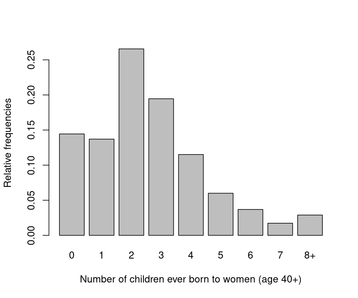
Figure 1.1: Fertility Distribution
We could use this data to answer questions like: is there a downward trend in fertility? If there is, can it be partially attributed to rising education levels? Note that here we only provide statistical explanation, and no casual analysis, meaning we do not aim to establish a cause-and-effect relationship. However, scientific studies suggest that education does have a casual effect on fertility. Economists propose that this effect is (partly) due to education raising the opportunity costs of not participating in the labor force. It might also be the case that more educated women make different life decisions that affect fertility rates. We can then return to the data and investigate whether average levels of fertility decreased, and average levels of education increased.
library("lattice")
trellis.par.set(theme = canonical.theme(color = FALSE))
print(xyplot(gss_zoo[,3:1], type = "b", xlab = "Year"))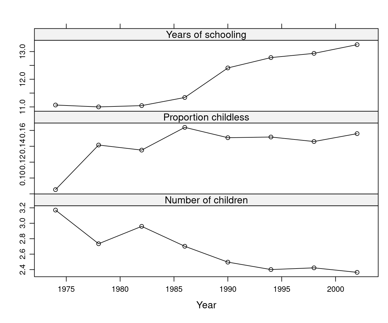
Figure 1.2: Trend in Education, Childlessness, and Number of Children
1.5.2 Secondary school choice
In Germany, students are separated relatively early, after 4 years of primary school, into three types of secondary school: Hauptschule (lower), Realschule (middle) and Gymnasium (upper). This placement seriously affects future education and labor market prospects, as only Gymnasium provides access to universities. Critics of this system point out that tracking takes place too early, and is strongly influenced by parents both directly and indirectly, which potentially results in maintained educational differences over generations. The data for our empirical analysis comes from the German Socio-Economic Panel (GSOEP), first collected in 1984. Here we use a selected sample of 675 14-year-old children born between 1980 and 1988. The variable of interest – school choice – can be regarded as a multinomial or ordered variable.
data("GSOEP9402", package = "AER")
levels(GSOEP9402$school)[3] <- "Gymn."
plot(school ~ meducation, data = GSOEP9402,
  breaks = c(7, 9, 10.5, 11.5, 12.5, 15, 18),
  xlab = "Mother's education", ylab = "School track of child")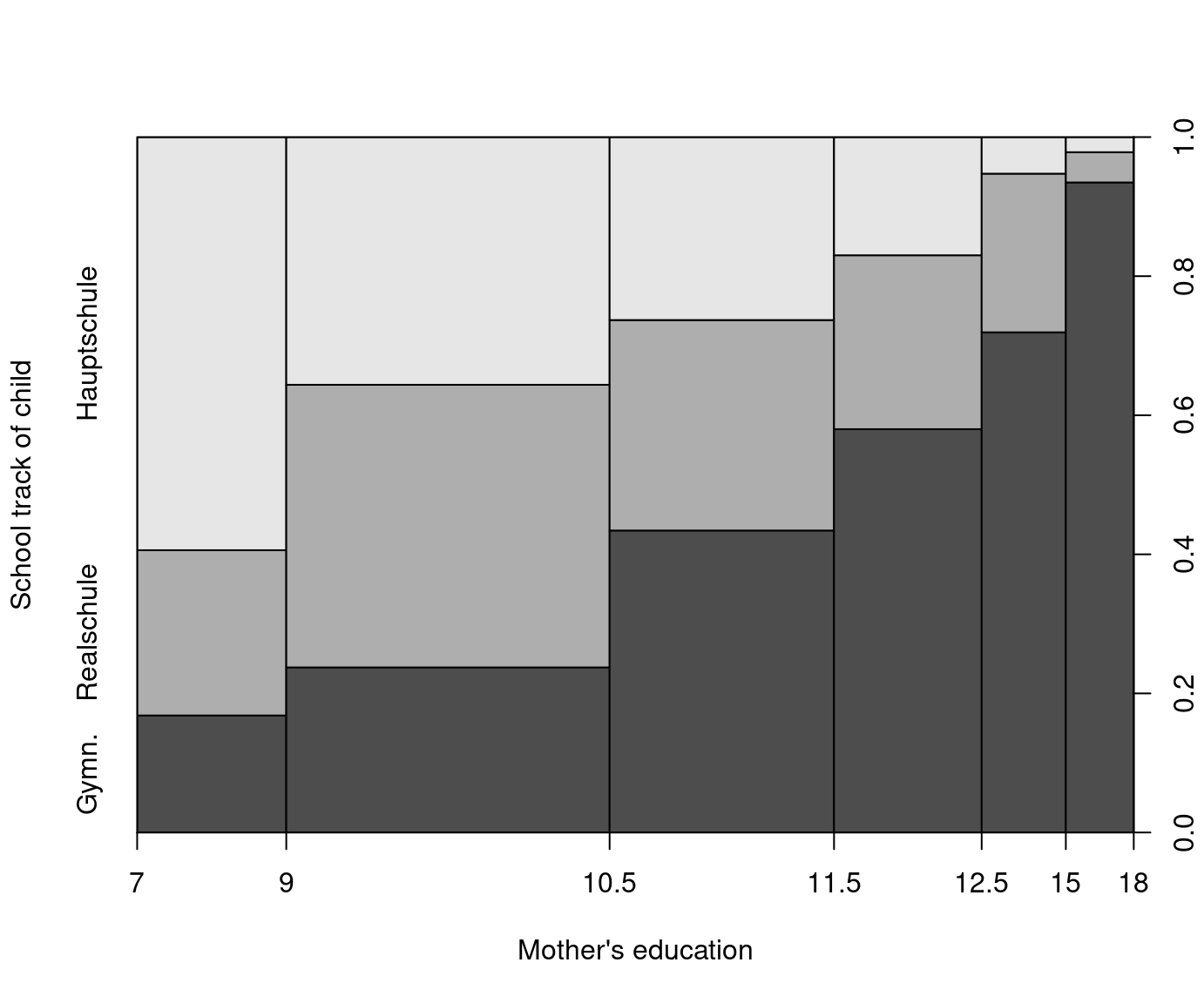
Figure 1.3: Mother’s Education and School Track of Child
1.5.3 Female hours of work and wages
Our third and final example in this chapter is determinants of women’s labor supply, a widely studied topic. We use cross-section data from the 1976 Panel Study of Income Dynamics (PSID), based on data from 1975. The topic (with this dataset) was famously investigated by Mroz (1987, Econometrica). The dataset contains a sample of 753 married women, out of whom 428 worked, and 325 did not. The number of hours worked (among working women) ranged from 12 to 4,950 hours, with an average of 1,303 hours per year, which is \(\approx\) 27 hours per week, counting with 48 working weeks. The average hourly wage of working women was 4.20 USD. The data also include several explanatory variables, such as age, education level, previous labor market experience, husband’s income, and the presence of young and adolescent children in the household.
data("PSID1976", package = "AER")
PSID1976$nwincome <- with(PSID1976, (fincome - hours * wage)/1000)
plot(hours ~ nwincome, data = PSID1976,
  xlab = "Non-wife income (in USD 1000)",
  ylab = "Hours of work in 1975")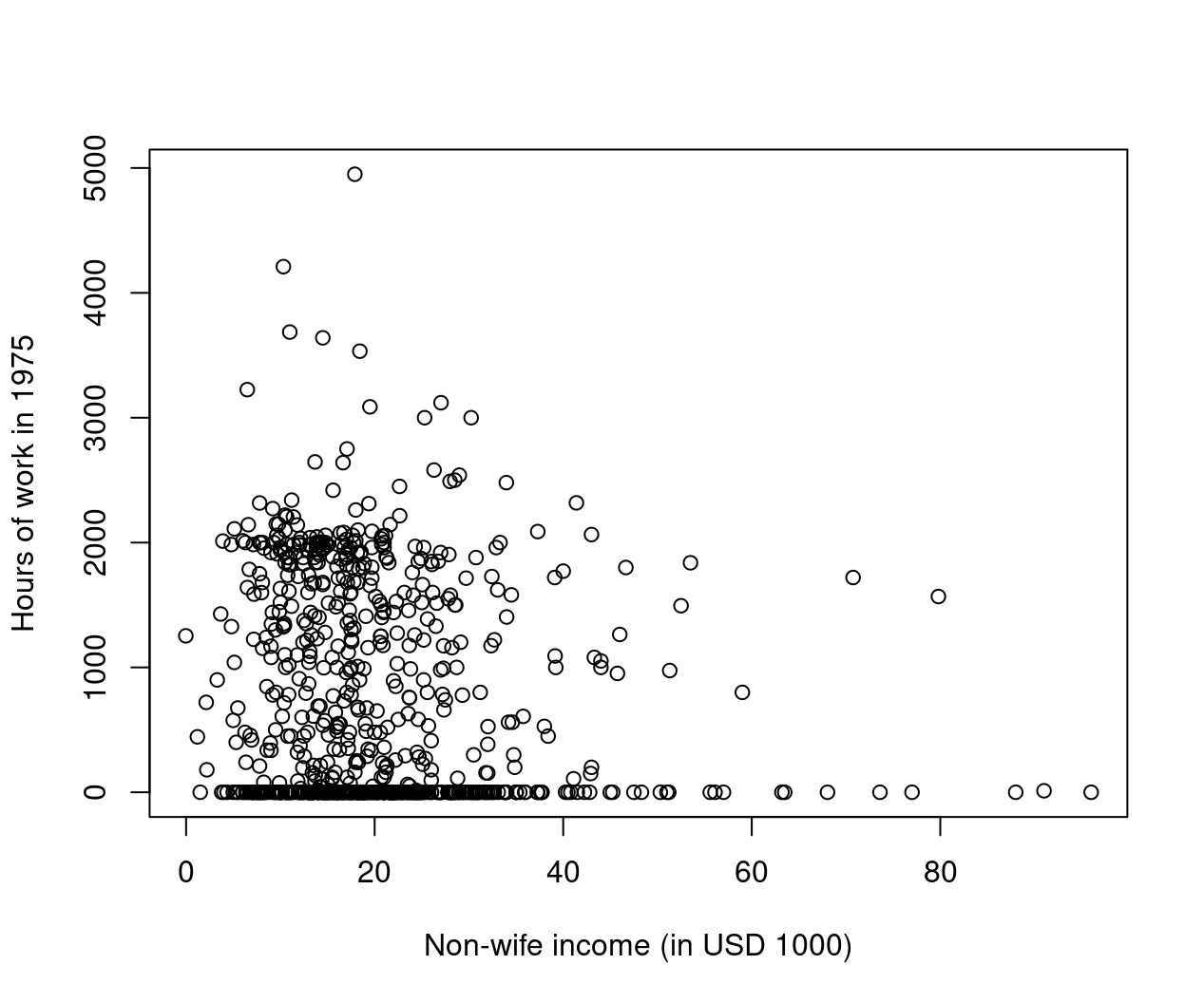
Figure 1.4: Non-Wife Income and Hours of Work in 1975
plot(jitter(hours, 200) ~ jitter(wage, 50), data = PSID1976,
  xlab = "Wife's average hourly wage (jittered)",
  ylab = "Hours of work in 1975 (jittered)")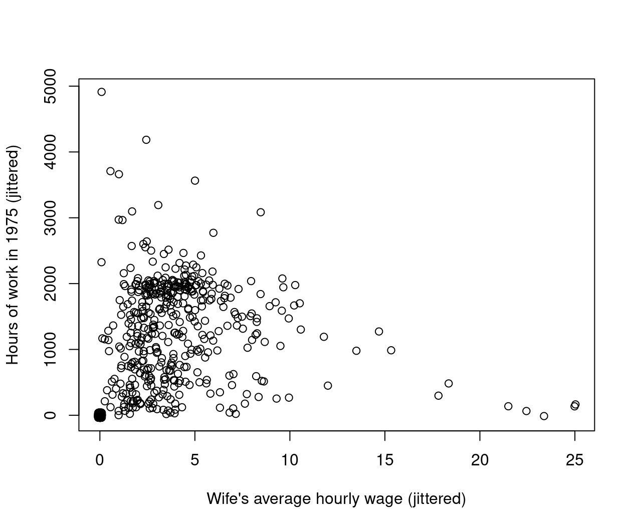
Figure 1.5: Hourly Wage and Hours of Work in 1975