Chapter 5 Semiparametric regression
5.1 Univariate smoothing
This chapter discusses the problem of estimating an unknown functional relationship between some response \(y\) and a continuous covariate \(z\). Note that in the upcoming we distinguish between covariates that enter the model linearly, denoted by \(x\), and as nonlinear model terms, denoted by \(z\) respectively. The representation of smooth functions is best introduced considering the following model: \[ y_i = f(z_i) + \varepsilon_i \] where \(f( \cdot )\) is a smooth function and \[ E(\varepsilon_i) = 0 \,\, \text{and} \,\, Var(\varepsilon_i) = \sigma^2. \] For the moment we assume that the errors are \[ \varepsilon_i \overset{i.i.d.}{\sim} N(0, \sigma^2). \]
The R package MASS contains a data set that is often used as an illustration in semiparametric regression.
data("mcycle", package = "MASS")
par(mar = c(4.1, 4.1, 0.1, 0.1))
plot(mcycle)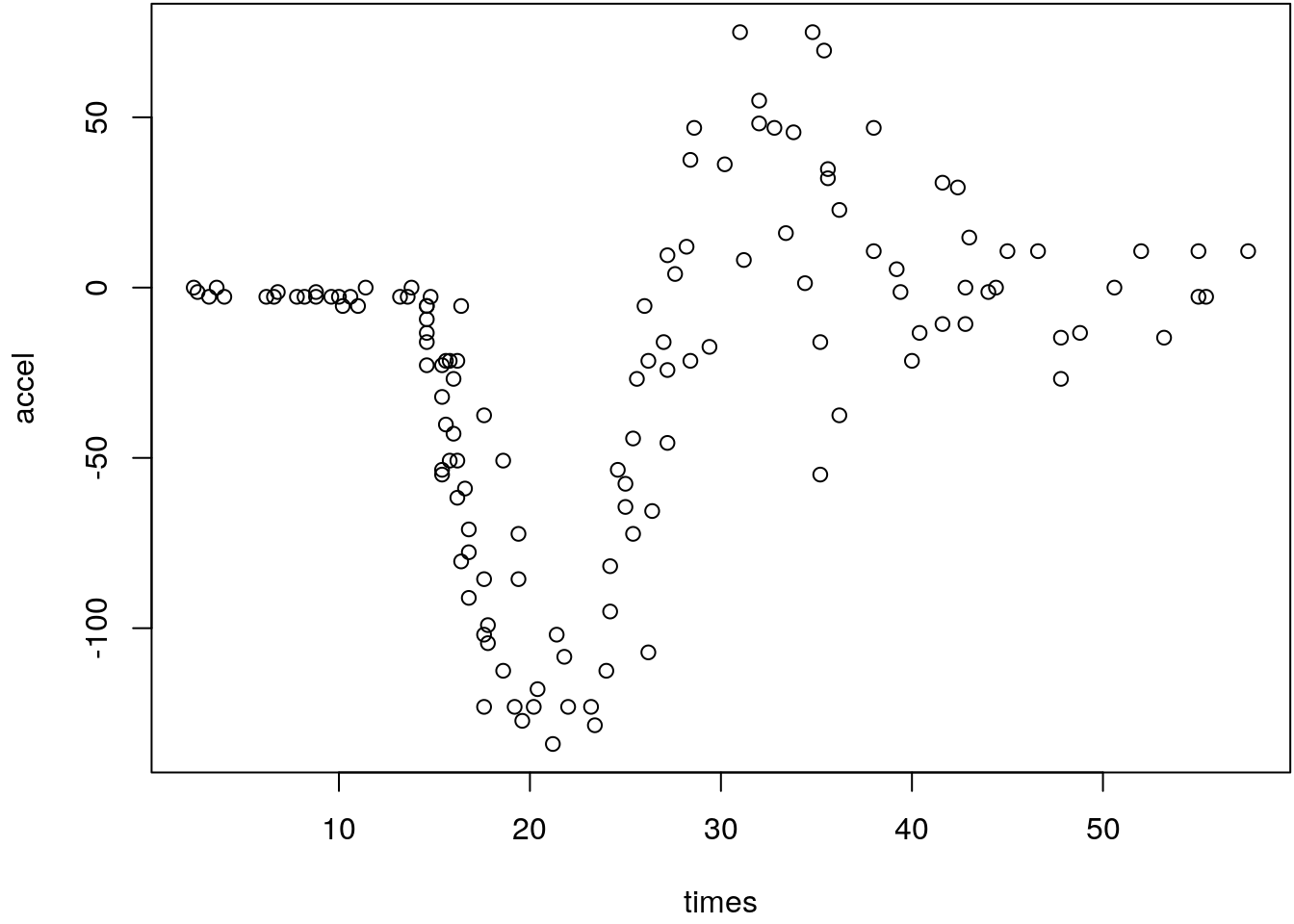
The data contain measurements of the head acceleration (in \(g\), variable accel) in a
simulated motorcycle accident (Silverman 1985), recorded in milliseconds after impact
(variable times). Clearly, the scatterplot indicates that a simple linear model will not
approximate the nonlinear relationship.
Polynom splines
We have already learned, that polynomial splines are a useful tool for the estimation of nonlinear relationships, see section Polynomial regression.
So if a linear fit is too simple we could use a polynomial model \[ \texttt{accel}_i = \gamma_0 + \gamma_1\texttt{times}_i + \ldots + \gamma_l\texttt{times}_i^l. \]
- The parameters can be estimated by ordinary least squares. Note that for nonlinear modelled terms parameters are always represented by \(\gamma_j\), linear model terms remain with \(x_j\beta_j\).
- Note that we write \(\gamma\) instead of \(\beta\) to better distinguish between simple linear and nonlinear effects here.
- The design matrix has the following form \[ \mathbf{Z} = \begin{pmatrix} 1 & \texttt{times}_1 & \dots & \texttt{times}_1^l \\ \vdots & \vdots & \vdots & \vdots \\ 1 & \texttt{times}_n & \dots & \texttt{times}_n^l \end{pmatrix} \]
- The columns of \(Z\) are also called basis functions \(B_j(z)\), \(j = 0, \ldots, l\). In this case a polynomial basis. Note that in the following \(\mathbf{Z}\) always represents a design matrix for nonlinear modelled terms.
- With sorted \(z\) they have a nice visual representation.
par(mar = c(4.1, 4.1, 0.1, 0.1))
z <- seq(-1, 1, length = 100)
Z <- outer(z, 0:3, "^")
matplot(x = z, y = Z, type = "l", lty = 1, col = 1:ncol(Z),
  lwd = 2, ylab = expression(B[j](z)))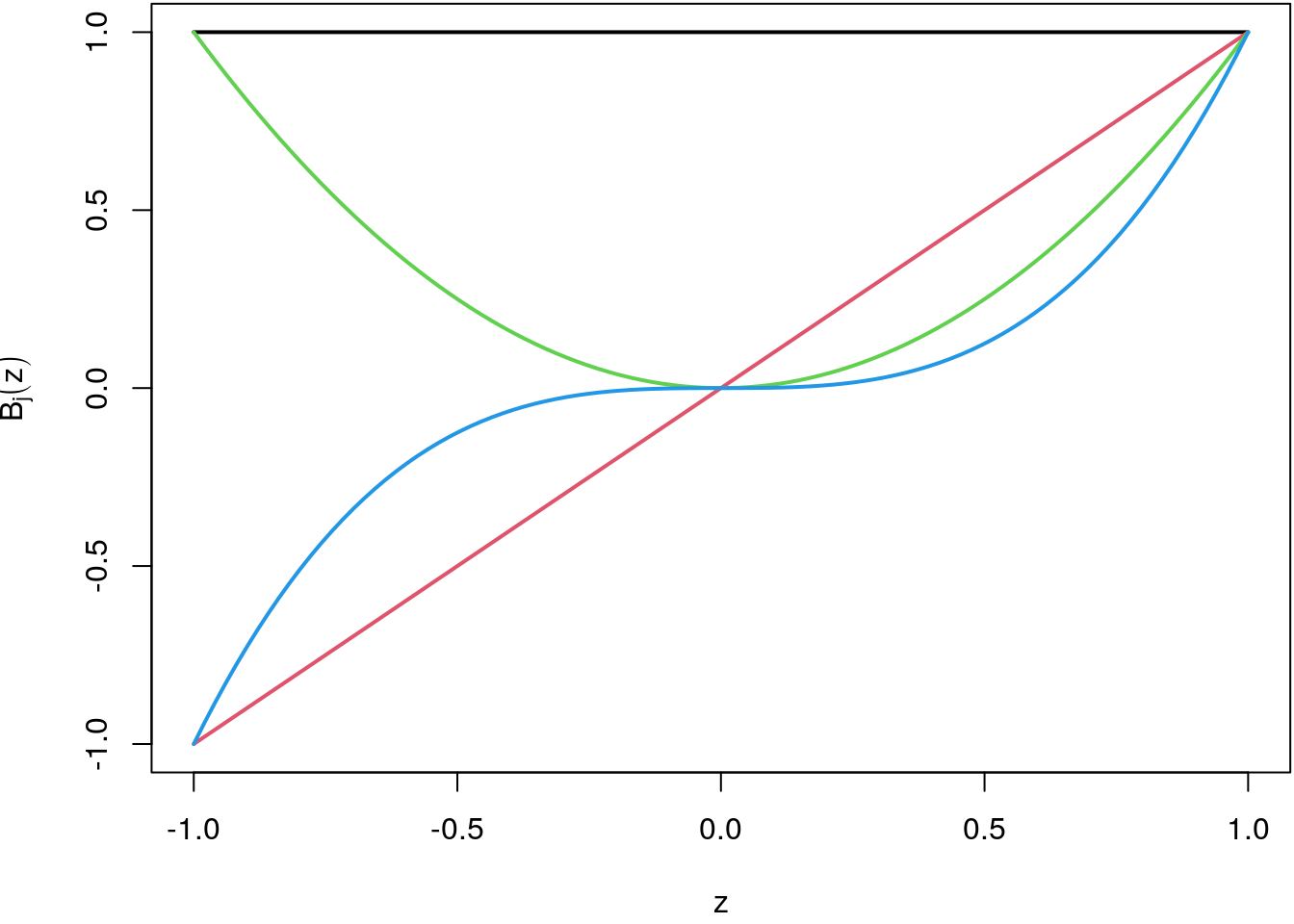
The black line is the polynomial transformation of degree 0, the red line of degree 1 (identity
transformation), the green line of degree 2 and the blue line represents degree 3. In a regression
setting each of the basis functions in \(\mathbf{Z}\), the columns, are scaled with the corresponding
regression coefficients \(\gamma_j\). The sum of all scaled basis function then results in the
approximated smooth function. This is illustrated in the following graphic:
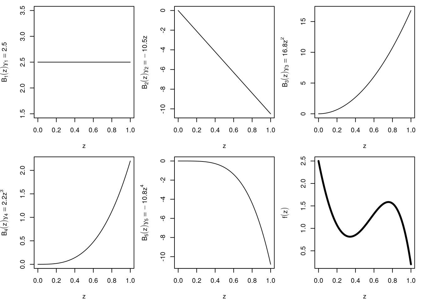
In this example 5 basis functions \(B_j( \cdot )\) are scaled with their respective coefficients \(\gamma_j\). The final curve shown in the lower right panel is just the linear combination of basis functions and regression coefficients \[ f(z) = \sum_{j = 1}^5 B_j(z)\gamma_j. \]
As already mentioned it is not very good to create the columns of the design matrix of the
polynomial regression model by simple power transformation. It is much more numerically stable
to use orthogonal polynomials instead. In R orthogonal polynomials can be computed with
function poly() (see also Polynomial regression). Now let’s
try polynomial regression in the simulated motorcycle accident data example. We fit a number
of different polynomials and see if we can approximate the nonlinear relationship.
par(mar = c(4.1, 4.1, 0.1, 0.1))
plot(mcycle)
degree <- c(1, 2, 6, 9, 15)
for(i in seq_along(degree)) {
  b <- lm(accel ~ poly(times, degree[i]), data = mcycle)
  lines(fitted(b) ~ times, col = i, data = mcycle, lwd = 2)
}
legend("bottomright", paste("l =", c(1, 2, 6, 9, 15)),
  lwd = 2, col = 1:i, bty = "n")
The graphic clearly shows that polynomial regression cannot approximate the complex nonlinear
relationship. Even polynomials up to \(l = 15\) lead to an unsatisfactory fit, since the
boundary problems at the borders of the domain of variable times become larger and larger.
So basically we are faced with the following problems:
- High degree needed for decent curve fit.
- Polynomial basis functions are global.
- Hence, polynomial regression models suffer from unexpected wiggles.
In summary, we cannot approximate such complex relationships with ordinary polynomial models, we need something better.
One simple idea to overcome these problems is to divide the domain of the covariate into separate intervals defined by so called knots \(\boldsymbol{\kappa}\) and to estimate a low degree polynomial model within each section. This is illustrated in the following:
par(mar = c(4.1, 4.1, 0.1, 0.1))
steps <- mcycle$times[c(1, 25, 96, 133)]
plot(mcycle)
for(i in 2:length(steps)) {
  z <- with(mcycle, times[steps[i - 1] <= times & times <= steps[i]])
  y <- with(mcycle, accel[steps[i - 1] <= times & times <= steps[i]])
  b <- lm(y ~ z + I(z^2) + I(z^3))
  lines(z, fitted(b))
}
abline(v = steps, lty = 2)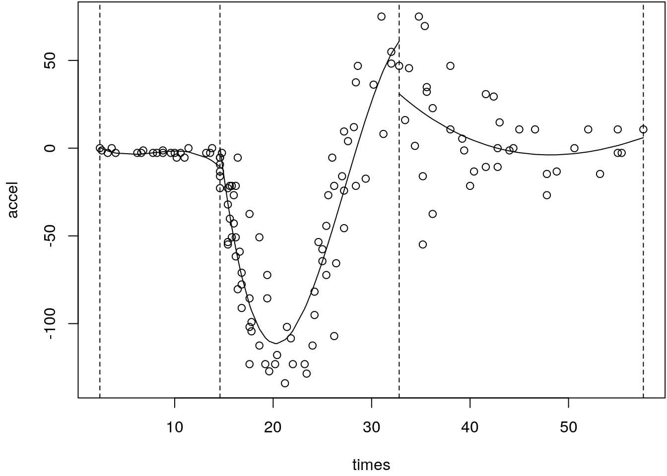
This little trick already gives a good approximation of the functional relationship, however:
- The fitted functions don’t form a nice overall smooth function, see the jumps at the boundaries.
- We need additional requirements to construct a smooth functional form.
So we want an overall smooth function without jumps, therefore we need to ensure that the derivatives of the smooth function exist.
A function \(f( \cdot )\) is called polynomial spline of degree \(l \geq 0\) with knots \(min(z) = \kappa_1 < \ldots < \kappa_m = max(z)\) (the interval boundaries), if it satisfies
- \(f(z)\) is \((l - 1)\) times continuously differentiable,
- \(f(z)\) is a polynom of degree \(l\) in each interval \([\kappa_j, \kappa_{j + 1})\).
Every spline may be represented by a linear combination of basis functions, i.e.
\[
f(z_i) = \gamma_1 \cdot B_1(z_i) + \gamma_2 \cdot B_2(z_i) + \ldots + \gamma_{l + m - 1} \cdot
B_{l + m - 1}(z_i).
\]
Polynom splines with truncated powers
The requirements on the derivatives of the spline function are actually easy to incorporate. Let’s have a look at the so called truncated power polynomial model \[ y_i = \gamma_1 + \gamma_2z_i + \ldots + \gamma_{l + 1}z_i^l + \sum_{j = 2}^{m - 1} \gamma_{l + j}(z_i - \kappa_j)_{+}^l + \varepsilon_i, \] where \[ (z_i - \kappa_j)_{+}^l = \begin{cases} (z_i - \kappa_j)^l & z_i \geq \kappa_j \\ 0 & \text{else.} \end{cases} \] The corresponding basis functions are given by \[\begin{align} & B_1(z_i) = 1, \quad B_2(z_i) = z_i, \,\,\, \ldots \,\,\, , \quad B_{l + 1}(z_i) = z_i^l, \\ & B_{l + 2}(z_i) = (z_i - \kappa_2)_{+}^l, \,\,\, \ldots \,\,\, , \quad B_k(z_i) = (z_i - \kappa_{m - 1})_{+}^l. \end{align}\]
Therefore, we get \[ y_i = f(z_i) + \varepsilon_i = \sum_{j = 1}^k \gamma_j B_j(z_i) + \varepsilon_i. \] And the corresponding design matrix is \[\begin{align} \mathbf{Z} &= \begin{pmatrix} B_1(z_1) & \ldots & B_k(z_1) \\ \vdots & & \vdots \\ B_1(z_n) & \ldots & B_k(z_n) \end{pmatrix} \\ &= \begin{pmatrix} 1 & z_1 & \ldots & z_1^l & (z_1 - \kappa_2)_{+}^l & \ldots & (z_1 - \kappa_{m - 1})_{+}^l \\ \vdots & & & & & & \vdots \\ 1 & z_n & \ldots & z_n^l & (z_n - \kappa_2)_{+}^l & \ldots & (z_n - \kappa_{m - 1})_{+}^l \end{pmatrix}, \end{align}\]
Hence, the model can be estimated by least squares: \[ \mathbf{y} = \mathbf{Z}\boldsymbol{\gamma} + \boldsymbol{\varepsilon} \,\,\, \text{and} \,\,\, \hat{\boldsymbol{\gamma}} = (\mathbf{Z}^\top\mathbf{Z})^{-1}\mathbf{Z}^\top\mathbf{y}. \]
The following figure illustrates the truncated power series spline estimator on
the simulated motorcycle accident data:
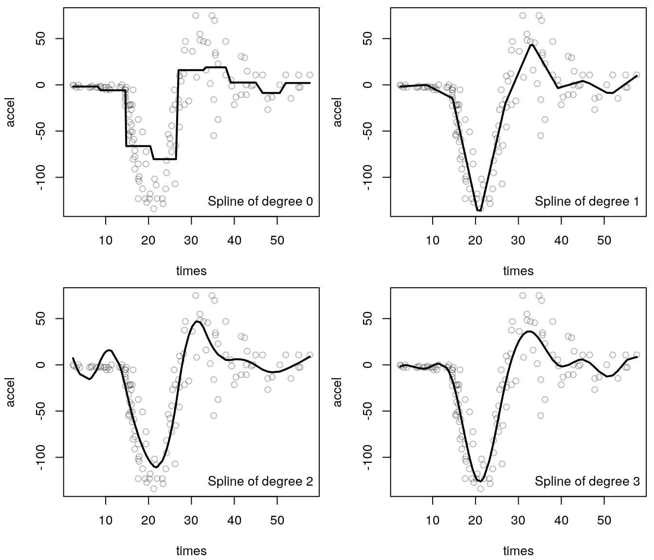
The splines are all based on 15 knots. The upper left panel shows that already a truncated power spline of degree 0 can approximate the nonlinear relationship quite well. By increasing the order of the polynomial we can capture the bottom spike better and better. Overall, a polynomial of degree 3 seems to provide a quite good fit.
To illustrate the estimation process in more detail, the following graphic shows the individual
steps using a truncated power basis of degree 1.
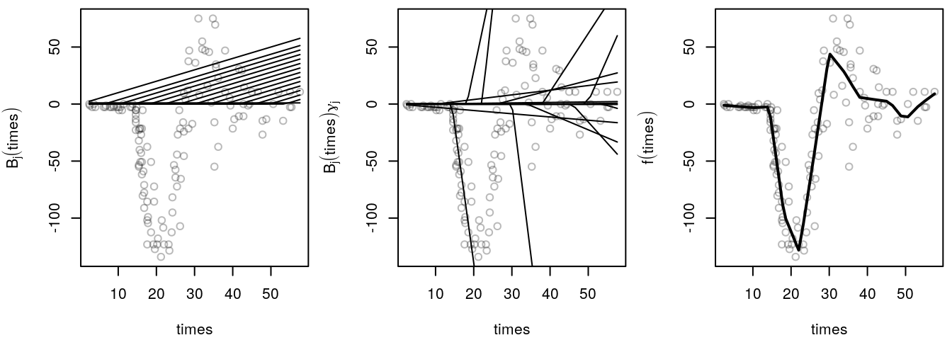
First, the basis functions are set up, this is shown in the left panel. Then, the basis functions are scaled with the corresponding regression coefficients, middle panel. The sum of all scaled basis function results in the smooth function estimate and is shown in the right panel.
Exercise 5.1 Set up a function tp() with arguments
tp(z, degree = 3, knots = seq(min(z), max(z), length = 10))that returns a design matrix of basis functions of a polynomial spline with truncated
powers representation. Argument z is the covariate used to set up the design matrix,
degree is the maximum degree of the polynomial and knots are the knots that
split up the range of z in intervals, default is 9 intervals with 10 equidistant
knots.
mcycle data from the MASS package, estimate models with varying degree of the
polynomial of the truncated power basis. Find the best fitting model using the Akaike information
criterion (AIC, function AIC()).
The tp() function can be implemented with
tp <- function(z, degree = 3, knots = seq(min(z), max(z), length = 10)) {
  ## If knots is integer.
  if(length(knots) < 2)
    knots <- seq(min(z), max(z), length = knots)
  ## Setup the columns for the global polynomials.
  Z <- outer(z, 0:degree, "^"); cn <- paste("z^", 0:degree, sep = "")
  ## Compute local polynomials.
  if(length(knots) > 2) {
    knots <- sort(unique(knots))
    for(j in 2:(length(knots) - 1)) {
      zk <- z - knots[j]
      check <- zk < 0
      zk <- zk^degree
      zk[check] <- 0
      Z <- cbind(Z, zk)
      cn <- c(cn, paste("(z-", round(knots[j], 2), ")^", degree, sep = ""))
    }
  }
  ## Assign column names.
  colnames(Z) <- cn
  return(Z)
}
Now, search for the best degree of the polynomial,
degree <- 0:20
aic <- rep(0, length(degree))
for(i in seq_along(degree)) {
  b <- lm(accel ~ tp(times, degree = degree[i]) - 1, data = mcycle)
  aic[i] <- AIC(b)
}

## Re-estimate best fitting model.
i <- which.min(aic)
print(degree[i])
## [1] 3b <- lm(accel ~ tp(times, degree = degree[i]) - 1, data = mcycle)
p <- predict(b, interval = "confidence")
## Plot.
par(mfrow = c(1, 2), mar = c(4.1, 4.1, 0.5, 0.5))
plot(aic ~ degree, type = "l")
abline(v = degree[i], lty = 2, col = "lightgray")
plot(mcycle, col = rgb(0.1, 0.1, 0.1, alpha = 0.3))
matplot(mcycle$times, p, type = "l", lty = c(1, 2, 2),
add = TRUE, lwd = 1.5, col = 1)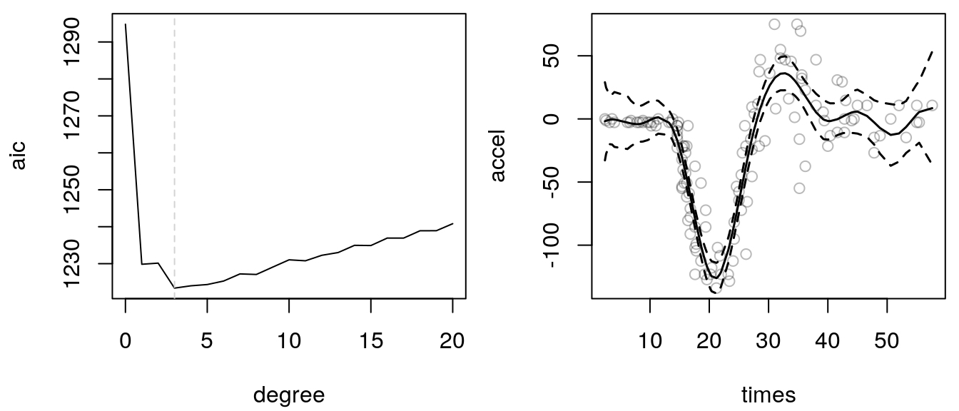
According the AIC a polynomial of degree 3 fits best. Looking
at the 95% credible intervals we see that for small times the intervals are too large. Hence,
again it seems that there is a heteroskedasticity problem. This topic will be discussed in
the upcoming chapters.
Knot selection
By searching for the degree of the polynomial we could definitely improve the model fit in the simulated motorcycle accident data example (see the last exercise). However, only looking at the degree of the polynomial might not be sufficient in a number of applications. The number of knots plays a much more important role for the approximation capability of the spline model.
But how many knots should be used and where should we place them? We could do the following:
- Equidistant knots. Compute \(h = (max(\mathbf{z}) - min(\mathbf{z})) / (m - 1)\), then the knots are \[ \kappa_j = min(\mathbf{z}) + (j - 1) \cdot h, \quad j = 1, \ldots, m. \]
- Quantile based knots. Choose the \[ (j - 1) / (m - 1)\text{-quantiles}, \quad j = 1, \ldots, m, \] of observations \(z_1, \ldots, z_n\).
- Visual inspection.
The following figure illustrates the effect of increasing the number of knots:
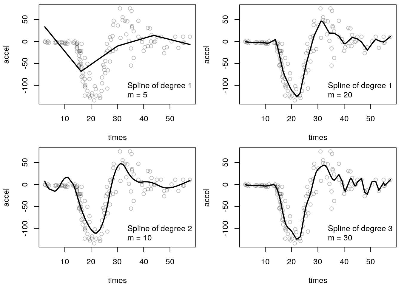
Clearly, the upper left panel indicates that the data cannot be approximated with a degree 1
polynomial and 5 knots. The fit is much more improved if we increase the number of knots to 20,
upper right panel. The lower left panel of a degree 2 polynomial with 10 knots shows actually
a quite good fit, the spikes could be modelled relatively good. However, for small values
of times the fitted line does not really approximate the data, it is simply too wiggly
in this area. Now, if we increase the degree to 3 and the number of knots to 30, we obtain a
very good fit for small values of times, but for large values the estimated function seem to
interpolate the data.
Automatic Selection – Knot Search Algorithm
A first naive way for selecting the number of equidistant intervals would be a simple grid search, i.e. for a certain maximum number of knots \(m\), choose the optimum number of knots \(\alpha \in \{2, \ldots, m\}\) that minimizes, e.g., the AIC. A function that implements the algorithm is only a couple of lines of code:
search.nknots <- function(y, z, IC = AIC, m = 50, ...) {
  knots <- 2:m; ic <- NULL
  for(i in knots)
    ic <- c(ic, IC(lm(y ~ -1 + tp(z, knots = i, ...))))
  return(knots[which.min(ic)])
}
The function has 4 arguments: y is the response variable, z is the covariate which should
be used for estimating a truncated power series spline. Argument IC is the information criterion
function that should be used for the selection step, the default is the AIC() function. Argument
m defines the maximum number of knots.
For example, using the mcycle data again we obtain
(k1 <- with(mcycle, search.nknots(accel, times, IC = AIC)))## [1] 11(k2 <- with(mcycle, search.nknots(accel, times, IC = BIC)))## [1] 7The resulting model fits can be visualized with
b1 <- lm(accel ~ -1 + tp(times, knots = k1), data = mcycle)
b2 <- lm(accel ~ -1 + tp(times, knots = k2), data = mcycle)

par(mar = c(4.1, 4.1, 0.1, 0.1))
plot(mcycle, col = rgb(0.1, 0.1, 0.1, alpha = 0.5))
lines(fitted(b1) ~ times, data = mcycle, col = 1)
lines(fitted(b2) ~ times, data = mcycle, col = 2)
legend("topleft", c("AIC", "BIC"), lwd = 1, col = 1:2, bty = "n")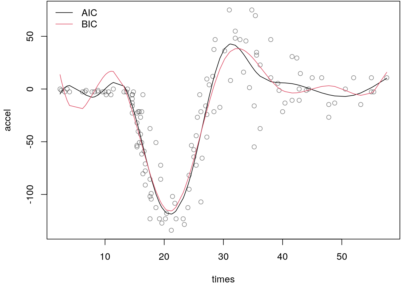
The plot indicates that both fitted curves model the relationship quite appropriate, however,
there are still problems for values of times smaller than 30. Here, the fitted lines are still
too wiggly and just don’t fit to the data. So there is still quite a lot of room for improvement.
5.1.0.1 Automatic Selection – MARS
An adaptive model selection algorithm is the so called stepwise regression. Here, in each step of the algorithm covariates may be dropped out from the model or enter the model according to some measure of goodness-of-fit. This is also called forward and backward elimination. In terms of semiparametric modeling this type of algorithm that selects the basis functions of a smooth model is also called multivariate adaptive regression splines (MARS). The Algorithm proceeds as follows.
Forward step:
- Create a full design matrix \(Z\).
- Start with the smallest possible model, i.e. start with the first column of \(Z\) (intercept).
- Successively add basis functions \(B_j(z_i)\) (columns) that have not been used, one at a time.
- Choose the basis function which, e.g., minimizes the RSS the most to be added to the model.
- Calculate an information criterion from the current model.
- Repeat 3.-5. until all basis functions are included in the model.
Backward step:
- Take the full design matrix \(Z\).
- Successively remove basis functions \(B_j(z_i)\) (columns) that have not been removed yet, one at a time.
- Choose the basis function which, e.g., maximizes the RSS the most to be removed from the model.
- Calculate an information criterion from the current model.
- Repeat 2.-4. until one basis function is left in the model.
Finally, choose the set of basis functions that minimizes the information criterion obtained from the forward and backward runs.
The analogy to stepwise regression is immediately apparent. Function step() implements
this type of algorithm for general linear models. With a little tweak we can use the implementation
to implement the MARS algorithm:
mars <- function(y, z, degree = 3, knots = 60,
  k = log(length(y)), ...)
{
  Z <- tp(z, degree, knots)
  colnames(Z) <- paste("z", 1:ncol(Z), sep = "")
  f <- paste("y", paste(c("-1", colnames(Z)), collapse = "+"),
    sep = "~")
  f <- as.formula(f)
  d <- cbind("y" = y, as.data.frame(Z))
  b <- step(lm(f, data = d), k = k, trace = FALSE, ...)
  b$model <- cbind(b$model, "zterm" = z)
  class(b) <- c("mars", "lm")
  return(b)
}
The function has arguments y, the response, z the covariate, degree is the degree
of the truncated power polynomial, knots defines the maximum number of knots and k defines
the penalty to the log-likelihood which defaults to the BIC criterion. We assign class "mars"
and "lm" to the returned object. The reason is that this way we can easily implement a nice
plotting method.
plot.mars <- function(x, add = FALSE, ...)
{
  mf <- model.frame(x)
  y <- mf[, 1]
  z <- mf$zterm
  if(!add)
    plot(z, y, ...)
  i <- order(z)
  p <- predict(x, se.fit = TRUE,
    interval = "confidence", type = "response")
  pol <- rbind(
    cbind(z[i], p$fit[i, "lwr"]),
    cbind(rev(z[i]), rev(p$fit[i, "upr"]))
  )
  polygon(pol, col = rgb(1, 0.55, 0, alpha = 0.5), border = NA)
  lines(p$fit[i, "fit"] ~ z[i])
  invisible(NULL)
}
Let’s see the algorithm in action again using the mcycle data set.
## AIC penalty.
b1 <- with(mcycle, mars(accel, times, k = 2))
print(coef(b1))
## z15 z17 z18 z19 z20 z21
## -1.949370 11.421160 -29.791466 58.719246 -75.524601 48.494332
## z23 z25 z26 z28 z30 z32
## -21.094802 37.103135 -41.829918 26.231585 -29.959254 96.182020
## z33 z34 z35 z36 z37 z38
## -191.246624 221.344367 -202.651567 182.904481 -175.966074 198.280675
## z39 z40 z41 z42 z43 z47
## -322.747187 571.639787 -698.707550 480.321983 -146.980736 22.691857
## z48 z51 z52 z55
## -22.709258 20.848322 -17.428067 2.746471## BIC penalty.
b2 <- with(mcycle, mars(accel, times, k = log(nrow(mcycle))))
print(coef(b2))## z15 z19 z20 z21 z26 z32
## -1.0024843 14.8505293 -24.3854010 11.0129155 -0.9558205 0.6371340
## z41
## -0.1730202## Plot.
par(mfrow = c(1, 2))
plot(b1, xlab = "times", ylab = "accel", main = "AIC")
plot(b2, xlab = "times", ylab = "accel", main = "BIC")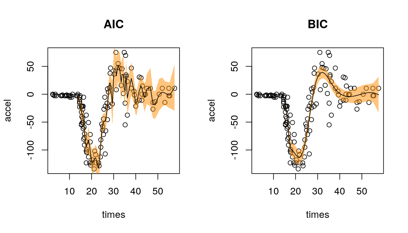
Here, using the AIC and BIC give quite different results. In total 28 basis functions are selected using the AIC and 7 with the BIC. Hence, the BIC selects a much sparser model and the AIC tends to overfit the data, which is also shown in the left panel. The estimated function using the BIC looks really well, each feature of the data seems to modelled quite appropriately. In addition, the 95% confidence intervals also follow the structure of the data for the first time (compare the results from the above).
Exercise 5.2 Using the MunichRent data, find the best fitting polynomial model
with the MARS algorithm
\[
\texttt{rentsqm}_i = \beta_0 + f(\texttt{yearc}_i) + \varepsilon_i,
\]
where function \(f( \cdot )\) is a polynomial of degree \(l\). Use the AIC and BIC for model
selection. Interpret the results.
The MunichRent data is loaded with
load("data/MunichRent.rda")Applying the MARS algorithm results
## AIC penalty.
b1 <- with(MunichRent, mars(rentsqm, yearc, k = 2))
print(coef(b1))
## z3 z22 z23 z24 z25
## 1.621541e-06 1.732071e+02 -6.536900e+02 8.799991e+02 -4.471016e+02
## z27 z28 z34 z39 z40
## 5.056848e+01 -2.995716e+00 2.548314e-02 -1.906349e-01 3.875147e-01
## z41 z44 z47 z48 z49
## -2.491446e-01 8.967693e-02 -6.298867e-01 1.657561e+00 -1.998849e+00
## z50 z52 z53 z54 z60
## 1.210217e+00 -8.033480e-01 8.193705e-01 -3.209605e-01 6.555189e-02## BIC penalty.
b2 <- with(MunichRent, mars(rentsqm, yearc, k = log(nrow(MunichRent))))
print(coef(b2))## z3 z27 z28 z34 z39
## 1.615163e-06 4.072725e-03 -5.178041e-03 1.898384e-03 -9.554744e-04## Plot.
par(mfrow = c(1, 2))
plot(b1, xlab = "yearc", ylab = "rentsqm", main = "AIC",
col = rgb(0.1, 0.1, 0.1, alpha = 0.1), cex = 0.3)
plot(b2, xlab = "yearc", ylab = "rentsqm", main = "BIC",
col = rgb(0.1, 0.1, 0.1, alpha = 0.1), cex = 0.3)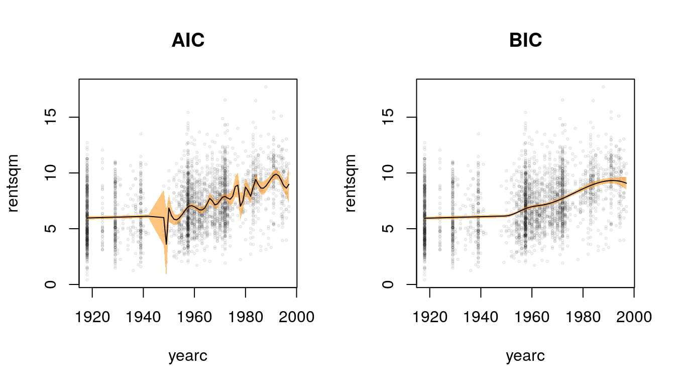
Also in this example, the MARS algorithm in combination with the AIC tends to overfit the data and provides quite wiggly estimates. The estimate with the BIC looks really well again. Rents seem to increase after the 1950s until about 1990 where there is a small decline visible.
Penalized regression
Although most of the automatic knot selection procedures exhibited good performance, they are usually quite complicated and computational intensive:
- We therefore seek a simpler method for flexible spline-based regression.
- As mentioned before, the roughness of a fit is due to there being too many knots in the model.
- Another way to overcome this problem is to retain all of the knots but to constrain their influence.
- The hope is that this will result in a less variable fit.
Now, consider the truncated polynomial model \[ f(z_i) = \gamma_1 + \gamma_2z_i + \ldots + \gamma_{l + 1}z_i^l + \sum_{j = 2}^{m - 1} \gamma_{l + j}(z_i - \kappa_j)_{+}^l. \] The wigglyness of the fit is mainly the result of too large variability of the coefficients of the truncated bases.
Constraints on the \(\gamma_{l+ j}\) that might rectify this situation are
- \(max|\gamma_{l + j}| < C\),
- \(\sum|\gamma_{l + j}| < C\), and
- \(\sum\gamma_{l + j}^2 < C\).
Each of these will lead to a smoother fit, however, the third constraint is much easier to implement. Therefore, define the \(((m - 2) + l) \times ((m - 2) + l)\) matrix \[ \mathbf{K} = \begin{pmatrix} \mathbf{0}_{l \times l} & \mathbf{0}_{l \times (m - 2)} \\ \mathbf{0}_{(m - 2) \times l} & \mathbf{I}_{(m - 2) \times (m - 2)} \end{pmatrix}, \] then our minimization problem can be written as \[ min ||\mathbf{y} - \mathbf{Z}\boldsymbol{\gamma}||^2 \,\,\, \text{subject to} \,\,\, \boldsymbol{\gamma}^\top\mathbf{K}\boldsymbol{\gamma} < C. \] Using a Lagrange multiplier argument, it can be shown that this is equivalent to choosing \(\gamma\) to minimize \[ ||\mathbf{y} - \mathbf{Z}\boldsymbol{\gamma}||^2 + \lambda\boldsymbol{\gamma}^\top\mathbf{K}\boldsymbol{\gamma} \] for some \(\lambda \geq 0\).
The solution is then given by \[ \hat{\boldsymbol{\gamma}} = \left(\mathbf{Z}^\top\mathbf{Z} + \lambda\mathbf{K}\right)^{-1} \mathbf{Z}^\top\mathbf{y}. \] The fitted values for a penalized spline regression are \[ \hat{\mathbf{y}} = \mathbf{Z}\left(\mathbf{Z}^\top\mathbf{Z} + \lambda\mathbf{K}\right)^{-1} \mathbf{Z}^\top\mathbf{y} = \mathbf{S}_{\lambda}\mathbf{y}, \] where \(\mathbf{S}_{\lambda}\) is called smoother matrix.
The influence of the smoothing parameter \(\lambda\) is illustrated in the following graphic:
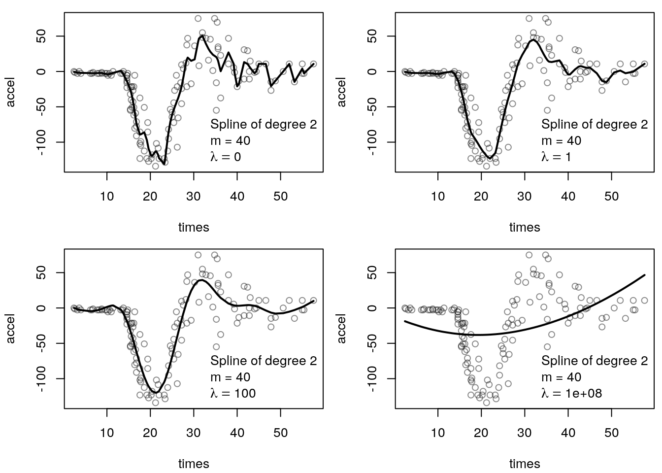
Penalizing the truncated power basis really seems to work, we obtain a quite good fit by setting \(\lambda = 10\). Clearly, increasing the smoothing parameter leads to smoother and smoother fits. In the extreme for very large values of \(\lambda\) the resulting curve is a polynomial of degree 2, since all truncated power basis functions are shrinked out of the model. This already illustrates a severe problem with the truncated power basis. In the limit, we would expect to see a linear function instead of a polynomial of degree 2.
This leads us to the next concept, the degrees of freedom of a smoother, or the equivalent number of parameters used to fit the model. If we can specify these in some way, we could easily implement a search algorithm that optimizes, e.g., the AIC or BIC to select the amount of shrinkage.
But let’s first summarize what we see in the above graphic
- A small value of \(\lambda\) leads to a wiggly scatterplot smooth, whereas a very large \(\lambda\) results in a parametric fit that depends on the degree of the spline basis functions.
- What is not so clear is the relationship between intermediate values of \(\lambda\) and the resulting amount of smoothing.
- In general, if we increase \(\lambda\) by 50% the fit does not get 50% smoother, we therefore need a more elaborate concept of describing the smoothness of a function.
So the value of the smoothing parameter does not have a direct interpretation as to how much structure is being imposed to the fit. A transformation \(t(\lambda)\) of \(\lambda\) that provides a reasonable solution to this problem is \[ t(\lambda) = trace(\mathbf{S}_{\lambda}), \] which is called the degrees of freedom of the fit corresponding to \(\lambda\). And since \[ trace(\mathbf{H}) = p = df, \] gives the equivalent degrees of freedom of the model fit, \(trace(\mathbf{S}_{\lambda})\) is a generalization of this definition for scatterplot smooths.
For a penalized spline smooth with \(m\) knots and degree \(l\), it is easily shown that \[ trace(\mathbf{S}_{0}) = l + m - 1. \] At the other extreme, \[ trace(\mathbf{S}_{\lambda}) \rightarrow l + 1 \,\,\, \text{as} \,\,\, \lambda \rightarrow \infty. \] So positive values of \(\lambda\) correspond to \[ l + 1 < df < l + m - 1. \]
Choosing the smoothing parameter
If \(\lambda\) is too high the data will be over smoothed, and if it is too low then the data will be under smoothed. In both cases, this means that the spline estimate \(\hat{f}\) will not be close to the true function.
Therefore, choose the smoothing parameter \(\lambda\), e.g., by cross validation, by using the AIC, BIC or the GCV criterion. For univariate regression models this could be done by a simple grid search, e.g., using the GCV:
## Setup the design and penalty matrix.
degree <- 2
Z <- tp(mcycle$times, degree = degree, knots = 40)
K <- diag(c(rep(0, degree + 1), rep(1, ncol(Z) - degree - 1)))

## Perform a simple grid search.
lambda <- seq(1e-03, 1e+03, length = 500)
gcv <- NULL
n <- nrow(mcycle)
ZZ <- crossprod(Z)
tZ <- t(Z)

## Run the search.
for(i in lambda) {
  S <- Z %*% solve(ZZ + i * K) %*% tZ
  yhat <- S %*% mcycle$accel
  trS <- sum(diag(S))
  rss <- sum((mcycle$accel - yhat)^2)
  gcv <- c(gcv, drop(rss * n / (n - trS)^2))
}

## Plot GCV curve and fitted smooth effect.
par(mfrow = c(1, 2), mar = c(4.1, 4.1, 0.5, 0.5))
plot(gcv ~ lambda, type = "l", lwd = 2)
i <- which.min(gcv)
abline(v = lambda[i], lty = 2, col = "lightgray")
plot(mcycle, col = rgb(0.1, 0.1, 0.1, alpha = 0.5))
S <- Z %*% solve(ZZ + lambda[i] * K) %*% tZ
yhat <- S %*% mcycle$accel
lines(yhat ~ mcycle$times, lwd = 2)
legend("bottomright", paste("df =", round(sum(diag(S)), 2)), bty = "n")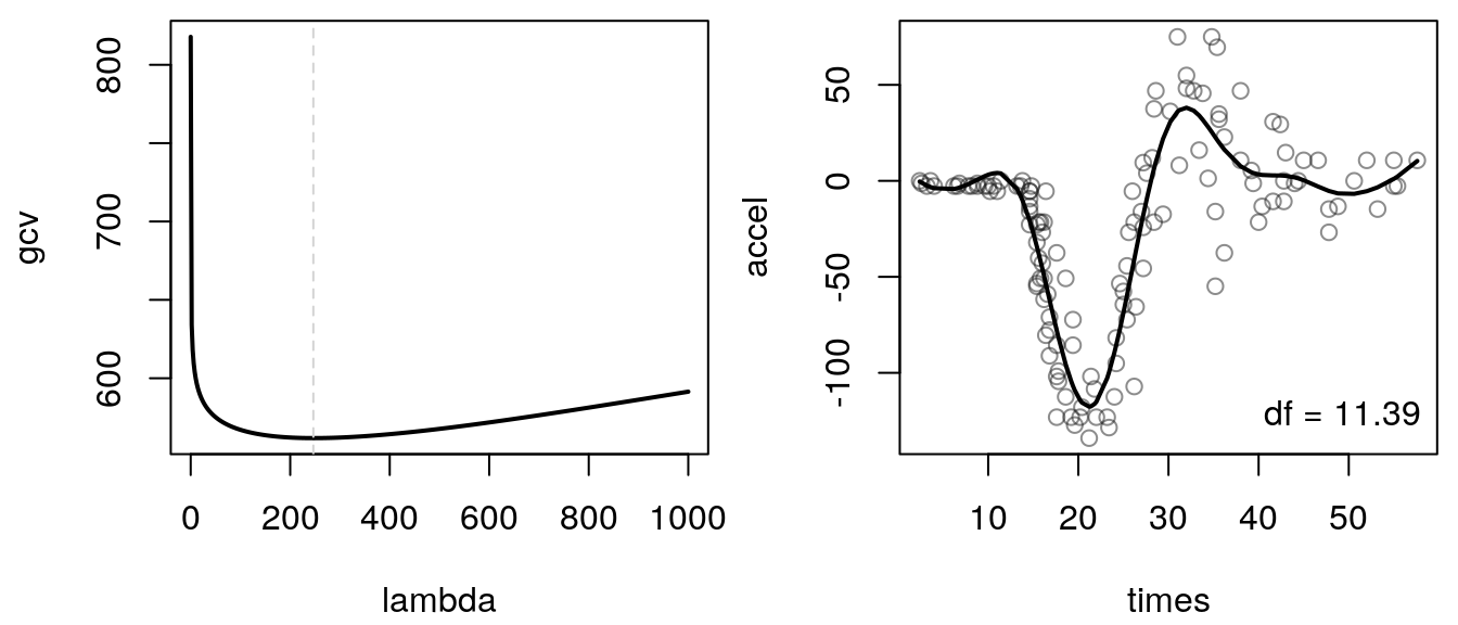
The grid search finds an optimum smooth parameter \(\lambda = 246.49\), which
results in a smooth function estimate with 11.39 degrees of freedom.
The fitted curve approximates the nonlinear relationship quite well, however, for values of
times smaller than 15 there is still some room for improvement, since the kink from zero
is not really captured as compared to the final fitted curve using the MARS algorithm. Hence,
truncated power polynomials are an easy way to set up smooth functions, however, since they
cannot approximate a perfect linear function and there are still some small problems when using
the penalization approach, we need other types of smooth terms that can handle this.
P-splines
As noted in the last section, there are some issues with truncated power polynomial splines. In addition to the described above, truncated power bases can sometimes lead to numerical instability when there is a large number of knots and the smoothing parameter is small. Therefore, in practical use it is advisable to work with equivalent bases with more stable numerical properties. The most common choice is the B-spline basis. B-spline basis can represent cubic splines (and also higher or lower orders). The advantage of B-splines is that they are strictly local – each basis function is only non-zero over \(l + 1\) adjacent knots.
To define a B-spline with \(k\) basis functions we need to set up \(m + l + 1\) knots \[ \kappa_1 < \kappa_2 < \ldots < \kappa_{m + l + 1}, \] where the interval over which the spline is to be evaluated is \([\kappa_{l + 1}, \kappa_k]\), i.e., the first and the last \(l\) knot locations are essentially arbitrary.
Every basis function overlaps with \(2l\) neighboring basis functions and is positive over \(l + 2\) neighboring knots. The B-spline is \(l - 1\) times continuously differentiable. A \(l\)th order B-spline is then represented by \[ f(z_i) = \sum_{j = 1}^k B_j^l(z_i)\gamma_j. \]
The B-spline basis functions are most conveniently defined recursively as follows: \[ B_j^l(z_i) = \frac{z_i - \kappa_j}{\kappa_{j + l} - \kappa_{j}}B_j^{l - 1}(z_i) + \frac{\kappa_{j + l + 1}- z_i}{\kappa_{j + l + 1} - \kappa_{j + 1}}B_{j + 1}^{l - 1}(z_i), \] where \[ B_j^0(z_i) = \begin{cases} 1 & \kappa_j \leq z_i < \kappa_{j + 1}, \\ 0 & \text{else.} \end{cases} \] A common choice is a cubic spline basis with \(l = 3\).
Using R we can implement the B-spline basis quite easily using recursive evaluation:
## Single basis functions.
bsbasis <- function(z, knots, j, degree) {
  if(degree == 0)
    B <- 1 * (knots[j] <= z & z < knots[j + 1])
  if(degree > 0) {
    b1 <- (z - knots[j]) / (knots[j + degree] - knots[j])
    b2 <- (knots[j + degree + 1] - z) /
      (knots[j + degree + 1] - knots[j + 1])
    B <- b1 * bsbasis(z, knots, j, degree - 1) +
      b2 * bsbasis(z, knots, j + 1, degree - 1)
  }
  B[is.na(B)] <- 0
  return(B)
}

## And the complete design matrix.
bs <- function(z, degree = 3, knots = NULL) {
  ## Compute knots.
  if(is.null(knots))
    knots <- 40
  if(length(knots) < 2) {
    step <- (max(z) - min(z)) / (knots - 1)
    knots <- seq(min(z) - degree * step,
      max(z) + degree * step, by = step)
  }

  ## Evaluate each basis function
  ## and return the full design matrix B.
  B <- NULL
  for(j in 1:(length(knots) - degree - 1))
    B <- cbind(B, bsbasis(z, knots, j, degree))
  return(B)
}
The following graphic visualizes B-spline basis functions for varying degrees and knots.
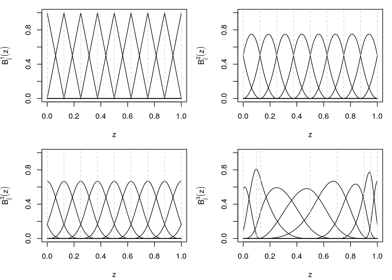
The upper left panel shows B-spline basis functions of degree 1 using an equidistant gird of knots, the upper right panel degree 2 B-spline basis functions and the lower left shows degree 3 B-splines basis. Not that the difference between degree 2 and 3 is quite small, a rule of thumb is to use degree 3 B-spline basis functions. The lower right panel then shows what happens to the basis functions for non-equidistant knots. Note that at the boundary of the domain of the covariate the basis functions are not complete. This is because we specified knots outside the domain of the covariate. This is illustrated in the next graphic.
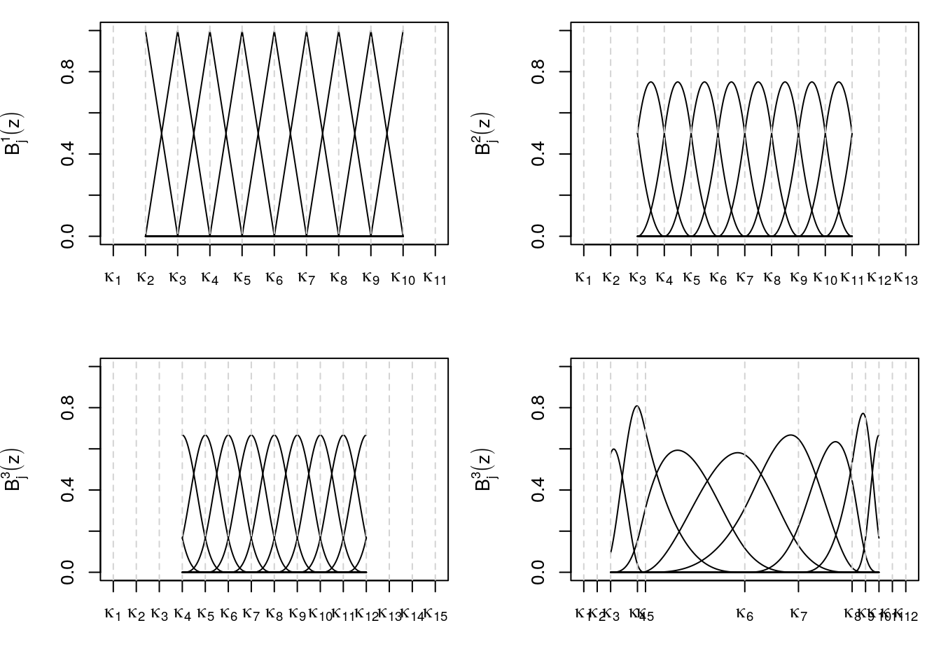
So the number of knots outside the domain of the covariate is dependent on the degree of the B-spline (see the definition above).
With B-spline basis functions a penalty on the regression coefficients is not obvious, since we do not divide in a parametric and non-parametric part. Because we want an overall smooth function we could use the following penalty \[ \lambda \int (f^{\prime\prime}(z))^2dz. \] For B-splines we can construct simpler equivalent penalty terms \[ ||\mathbf{y} - \mathbf{Z}\boldsymbol{\gamma}||^2 + \lambda\boldsymbol{\gamma}^\top\mathbf{K}\boldsymbol{\gamma} \] with \[ \lambda\boldsymbol{\gamma}^\top\mathbf{K}\boldsymbol{\gamma} = \sum_{j = k + 1}^k (\Delta^d \gamma_j)^2. \]
\(\Delta^d\) is the \(d\)th order difference which is defined recursively \[\begin{align} \Delta^1\gamma_j &= \gamma_{j} - \gamma_{j - 1} \\ \Delta^2\gamma_j &= \Delta^1\Delta^1\gamma_j = \Delta^1\gamma_j - \Delta^1\gamma_{j - 1} = \gamma_j - 2\gamma_{j - 1} + \gamma_{j - 2} \\ &\vdots& \\ \Delta^d\gamma_j &= \Delta^{d - 1}\gamma_j - \Delta^{d - 1}\gamma_{j - 1}. \end{align}\] The first order difference matrix is then given by \[ \mathbf{D}_1 = \begin{pmatrix} -1 & 1 & & & \\ & -1 & 1 & & \\ & & \ddots & \ddots & \\ & & & -1 & 1 \end{pmatrix} \,\,\, \text{with} \,\,\, \mathbf{D}_1\boldsymbol{\gamma} = \begin{pmatrix} \gamma_2 - \gamma_1 \\ \vdots \\ \gamma_k - \gamma_{k - 1} \end{pmatrix}. \] The penalty matrix can be set up with
P <- function(order = 2, k = 7) {
  D <- diag(k)
  for(i in 1:order)
    D <- diff(D)
  K <- crossprod(D, D)
  return(K)
}

## Order 1 penalty.
P(1)
## [,1] [,2] [,3] [,4] [,5] [,6] [,7]
## [1,] 1 -1 0 0 0 0 0
## [2,] -1 2 -1 0 0 0 0
## [3,] 0 -1 2 -1 0 0 0
## [4,] 0 0 -1 2 -1 0 0
## [5,] 0 0 0 -1 2 -1 0
## [6,] 0 0 0 0 -1 2 -1
## [7,] 0 0 0 0 0 -1 1## Order 2 penalty.
P(2)## [,1] [,2] [,3] [,4] [,5] [,6] [,7]
## [1,] 1 -2 1 0 0 0 0
## [2,] -2 5 -4 1 0 0 0
## [3,] 1 -4 6 -4 1 0 0
## [4,] 0 1 -4 6 -4 1 0
## [5,] 0 0 1 -4 6 -4 1
## [6,] 0 0 0 1 -4 5 -2
## [7,] 0 0 0 0 1 -2 1Exercise 5.3 Set up a function find.lambda() with arguments
find.lambda(y, Z, K)which minimizes the GCV score and returns the optimum smoothing parameter \(\lambda\). For optimization,
use the general purpose optimizer function optimize(). Then, find the optimum smooth parameter
in the mcycle example data using degree 3 P-splines with 80 knots.
The find.lambda() function can be implemented with
find.lambda <- function(y, Z, K) {
  ZZ <- crossprod(Z)
  tZ <- t(Z)

  gcv <- function(lambda) {
    S <- Z %*% solve(ZZ + lambda * K) %*% tZ
    yhat <- S %*% y
    trS <- sum(diag(S))
    rss <- sum((y - yhat)^2)
    drop(rss * n / (n - trS)^2)
  }

  lambda <- optimize(gcv, lower = 1e-20, upper = 1e+10)$minimum

  return(lambda)
}

## Set up design and penatly matrix.
Z <- bs(mcycle$times, degree = 3, knots = 80)
K <- P(2, ncol(Z))

## Search optimum lambda.
lambda <- find.lambda(mcycle$accel, Z, K)

## Estimate the function and plot.
S <- Z %*% solve(crossprod(Z) + lambda * K) %*% t(Z)
yhat <- S %*% y

par(mar = c(4.1, 4.1, 0.5, 0.5))
plot(mcycle, col =  rgb(0.1, 0.1, 0.1, alpha = 0.3))
lines(yhat ~ mcycle$times, lwd = 2)
legend("bottomright", paste("df =", round(sum(diag(S)), 2)), bty = "n")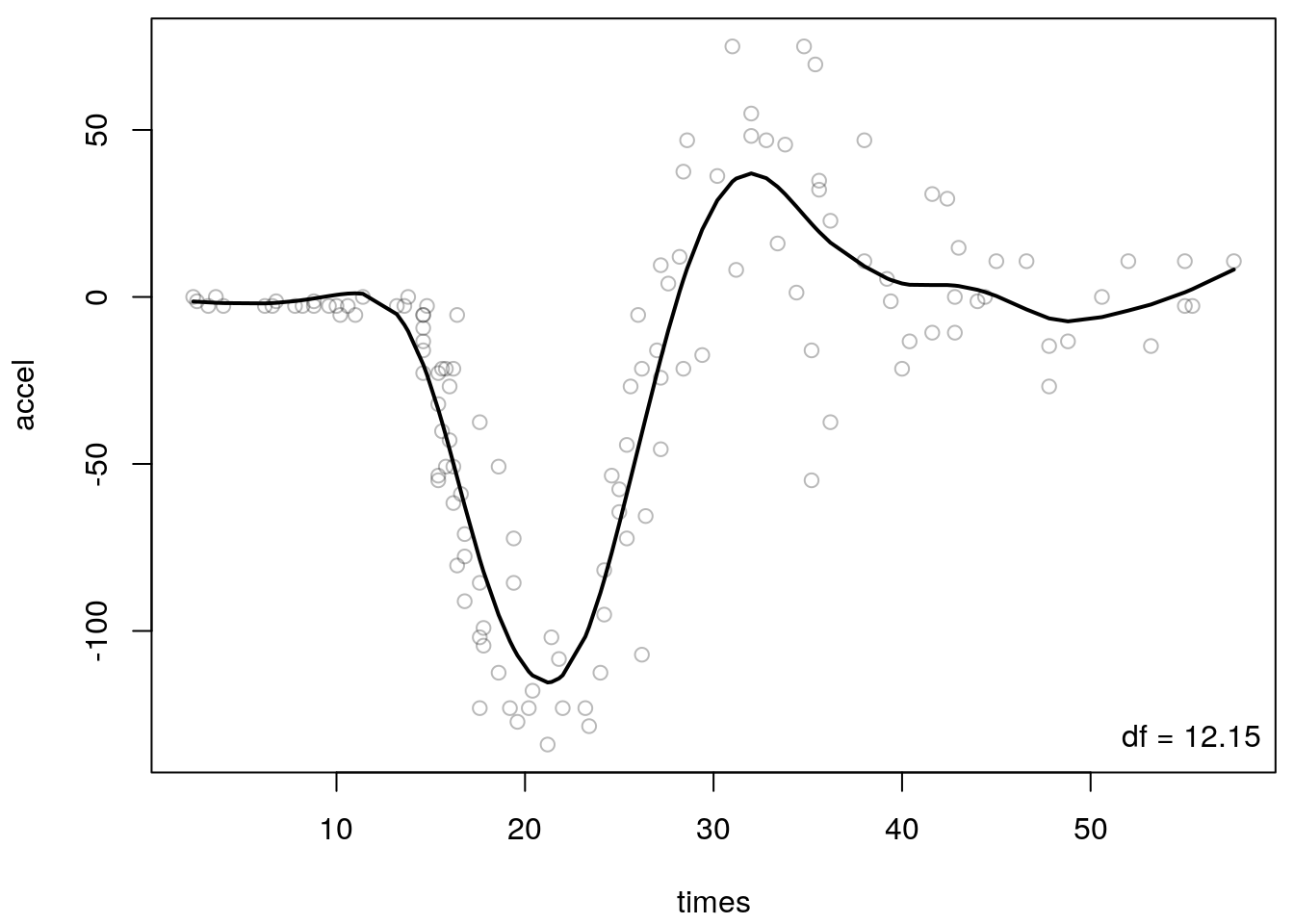
The estimated smooth function approximates the nonlinear relationship quite well, however,
there is still some room for improvement, as for the truncated polynomial splines, for small
values of times, since the function cannot model the kink perfectly. The estimated degrees
of freedom of the smooth of 12.15 is actually almost the same when
running the simple grid search with the truncated polynomial basis, see the example above.
5.2 Smooth additive models
This type of model is already introduced in section Additive models. The main difference here is that we setup the smooth functions using regression splines, which is much more flexible and superior in terms of out-of-sample performance.
The previous chapter showed how to construct flexible regression models for a single continuous predictor modeled as a smooth function, with all the other predictors entering the model linearly.
However, many regression problems involve several continuous covariates that may have nonlinear relationships with the response.
The extension to models that allow multiple smooth functions is relatively straightforward.
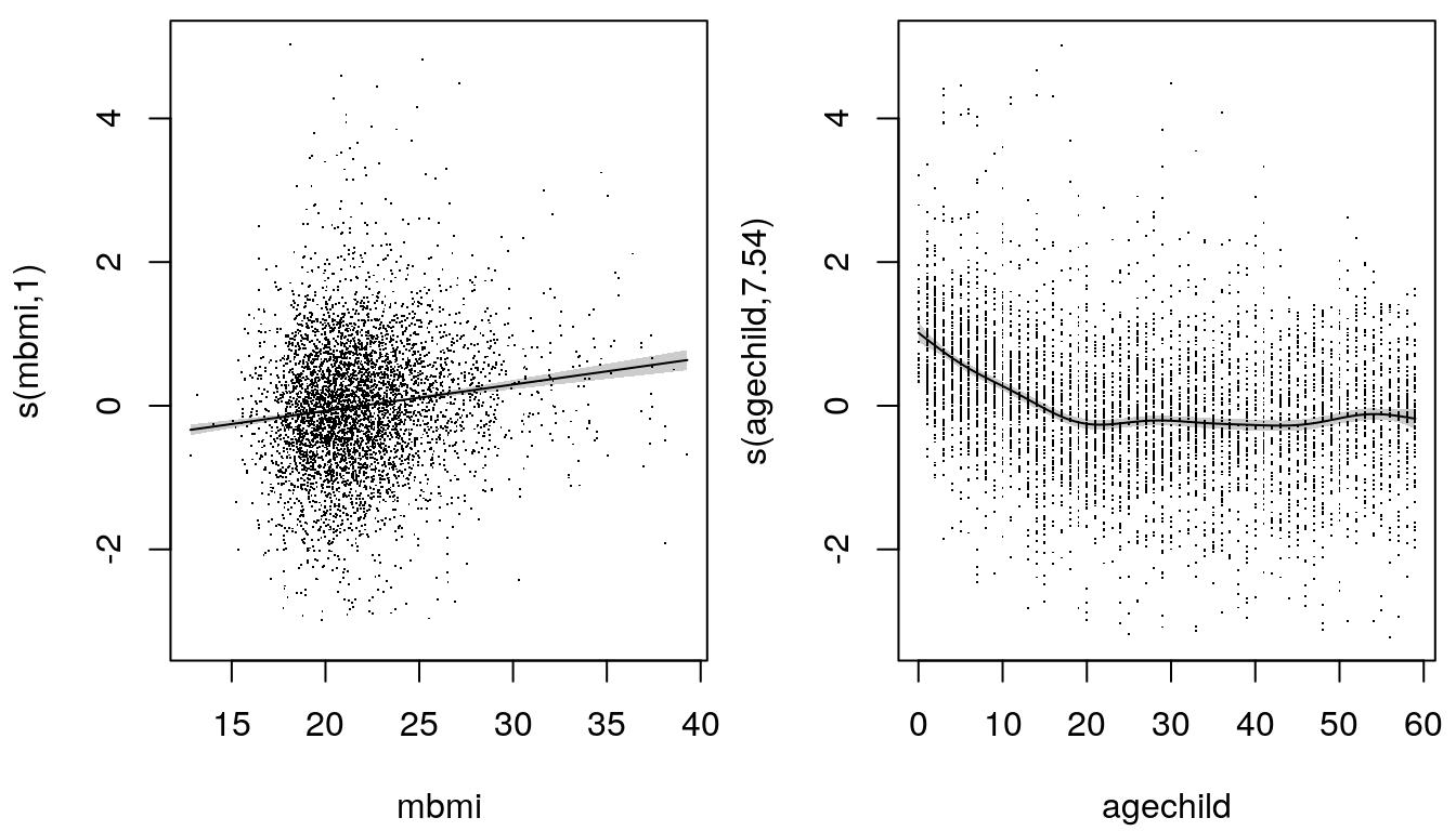
The following graphic gives an example of estimated effects from an additive model using the
ZambiaNutrition data.
Model definition
Consider observations \((y_i, x_{i1}, \ldots, x_{ik})\), \(i = 1, \ldots, n\), of a continuous response variable \(y\) and covariates \(x_1, \ldots, x_k\), whose effect on \(y\) can be modeled through a linear predictor.
Additionally, we have observations \((z_{i1}, \ldots, z_{iq})\), \(i = 1, \ldots, n\), of continuous covariates \(z_1, \ldots, z_q\) whose effects are to be modeled and analyzed nonparametrically. Additive models are defined by \[\begin{align} y_i &= f_1\left(z_{i1}\right) + \ldots + f_q\left(z_{iq}\right) + \beta_0 + \beta_1 x_{i1} + \ldots + \beta_k x_{ik} + \varepsilon_i \\ &= f_1\left(z_{i1}\right) + \ldots + f_q\left(z_{iq}\right) + \eta_i^{lin} + \varepsilon_i \\ &= \eta_i^{add} + \varepsilon_i, \end{align}\] with \[ \eta_i^{lin} = \beta_0 + \beta_1 x_{i1} + \ldots + \beta_k x_{ik},\qquad \eta_i^{add} = f_1\left(z_{i1}\right) + \ldots + f_q\left(z_{iq}\right) + \eta_i^{lin}. \]
There are two points to note about additive models. Firstly, the assumption of additive effects is a fairly strong one, e.g., \(f_1(z_1) + f_2(z_2)\) is a quite restrictive case of the general smooth function of two variables \(f(z_1, z_2)\).
Secondly, the fact that the model contains more than one function introduces an identifiability problem. If we add a constant \(c \not = 0\) to the function \(f_1(z_1)\) and subtract at the same time \(c\) from a second function \(f_2(z_2)\), the sum \[ f_1(z_1) + f_2(z_2) = f_1(z_1) + c + f_2(z_2) - c \] remains the same, i.e. the predictor \(\eta\) does not change if \(f_1(z_1)\) changes to \(\tilde{f}_1(z_1) = f_1(z_1) + c\) and \(f_2(z_2)\) changes to \(\tilde{f}_2(z_2) = f_2(z_2) - c\).
Although the functional form of \(f_1(z_1)\) and \(\tilde{f}_1(z_1)\) or \(f_2(z_2)\) and \(\tilde{f}_2(z_2)\) is unchanged, the overall level of the functions is arbitrary without imposing some further restrictions. Hence, it is necessary to fix the level of the functions. This is usually obtained by ``centering the functions around zero”, such that \[ \sum_{i=1}^n f_1(z_{i1}) = \ldots = \sum_{i=1}^n f_q(z_{iq})=0 \] holds.
Provided that the identifiability issue is addressed, the additive model can be represented using penalized splines, estimated by penalized least squares and the degree of the smoothing parameter selected by cross validation.
As with the linear model, the assumptions regarding the error variables \(\varepsilon_i\) carry over to the response variables \(y_i\), i.e. the \(y_i\) are (conditionally) independent with \[\begin{align} E(y_i) &= \mu_i = f_1(z_{i1})+ \ldots + f_q(z_{iq}) + \beta_0 + \beta_1 x_{i1} + \ldots + \beta_k x_{ik} \\ Var(y_i) &= \sigma^2 \end{align}\] and, if applicable, normally distributed with \[ y_i \sim N(\mu_i,\sigma^2). \]
The literature often refers the special case \[ y_i = f_1(z_{i1}) + \ldots + f_q(z_{iq}) + \varepsilon_i, \] without the additional linear predictor \(\eta_i^{lin}\) as the additive model.
Estimation
Each smooth function can be represented using a penalized regression spline basis, \(f_j\), \(j = 1, \ldots, q\), given by \[ f_j(z_j) = \sum_{l = 1}^{d_j} \gamma_{jl}B_l(z_j). \]
It is easy to see that the additive model can be written in linear model form \[ \mathbf{y} = \mathbf{Z}_1\boldsymbol{\gamma}_1 + \ldots + \mathbf{Z}_q\boldsymbol{\gamma}_q + \mathbf{X}\boldsymbol{\beta} + \boldsymbol{\varepsilon}. \]
The wiggliness of the functions can also be measured exactly as in the previous chapter \[ \boldsymbol{\gamma}_j^{\top}\mathbf{K}_j\boldsymbol{\gamma}_j. \]
The parameters of the model are obtained by minimization of the penalized least squares objective \[ ||\mathbf{y} - \mathbf{X}\boldsymbol{\beta} - \mathbf{Z}_1\boldsymbol{\gamma}_1 - \ldots - \mathbf{Z}_q\boldsymbol{\gamma}_q||^2 + \sum_{j = 1}^q \lambda_j \boldsymbol{\gamma}_j^{\top}\mathbf{K}_j\boldsymbol{\gamma}_j \]
To minimize we can choose between two alternatives: Iterative minimization using the backfitting algorithm, or direct minimization of the penalized least squares criterion.
The backfitting algorithm has the advantage that estimation of complex models can be traced back to one or two-dimensional smoothing.
In addition, the backfitting algorithm allows any combination of smoothers as building blocks for the estimation of additive models.
Backfitting
- Initialization: set, for example, \(\hat{\mathbf{f}}_1 = \ldots = \hat{\mathbf{f}}_q = \mathbf{0}, \hat{\boldsymbol{\beta}} = \mathbf{0}\).
- Obtain updated estimates \(\hat{\mathbf{f}}_j, j = 1, \ldots, q\), through \[ \hat{\mathbf{f}}_j = \mathbf{S}_j(\mathbf{y} - \sum_{l \not= j} \hat{\mathbf{f}}_l - \mathbf{X}\hat{\boldsymbol{\beta}}). \]
- Obtain updated estimates \(\hat{\boldsymbol{\beta}}\), through \[ \hat{\boldsymbol{\beta}} = (\mathbf{X}^{\top}\mathbf{X})^{-1}\mathbf{X}^{\top} (\mathbf{y} - \hat{\mathbf{f}}_1 - \ldots - \hat{\mathbf{f}}_q). \]
- Iterate the steps 2–3 until the estimated functions do not deviate more than a small given increment in two subsequent iterations.
Direct minimization
- We rewrite the additive model to \[ ||\mathbf{y} - \mathbf{Z}\boldsymbol{\gamma}||^2 + \lambda_1\boldsymbol{\gamma}^{\top}\mathbf{K}_1\boldsymbol{\gamma} + \ldots + \lambda_q\boldsymbol{\gamma}^{\top}\mathbf{K}_q\boldsymbol{\gamma}, \] where the \(i^{th}\) row of \(\mathbf{Z}\) is now \[ \mathbf{Z}_i = \left[1, x_{i1}, \ldots x_{ik}, B_{i11}, \ldots, B_{id_11}, B_{i12}, \ldots, B_{id_qq}\right]. \]
- Defining \(\mathbf{K} \equiv \lambda_1 \mathbf{K}_1 + \ldots + \lambda_q \mathbf{K}_q\) the objective can be rewritten as \[ ||\mathbf{y} - \mathbf{Z}\boldsymbol{\gamma}||^2 + \boldsymbol{\gamma}^\top\mathbf{K}\boldsymbol{\gamma} = \begin{vmatrix}\begin{vmatrix} \begin{bmatrix} \mathbf{y} \\ \mathbf{0} \end{bmatrix} - \begin{bmatrix} \mathbf{Z} \\ \mathbf{B} \end{bmatrix} \boldsymbol{\gamma} \end{vmatrix}\end{vmatrix}^2, \] where \(\mathbf{B}\) is any matrix square root such that \(\mathbf{B}^\top\mathbf{B} = \mathbf{K}\).
R package mgcv
Additive models can be estimated using the R package mgcv. The main model fitting function
is gam() and the most important arguments are:
gam(formula, family = gaussian(), data = list(),
  weights = NULL, subset = NULL, na.action, offset = NULL)
The setup is pretty much identical to the lm() or glm() function. The main difference
that we can really estimate additive models with the help of smooth constructors in the formula.
For example, a nonlinear smooth function of a covariate z can be modelled by
b <- gam(y ~ s(z), data = d)Per default function s() sets up so called thin-plate regression splines, a type of spline
that will be described later in this script. Actually, there are a number of different spline
smoothers implemented, for a detailed list see ?smooth.terms. For a very detailed introduction
on additive models and the mgcv implementation please see the book
Wood (2006). Generalized Additive Models: An Introduction with {R}.
But for the moment, this is not so interesting, instead we focus on how to estimate a full
additive model and how we can visualize the effects, or predict from new data. Therefore, we
again exemplify the model using the Munich rent index data MunichRent
and estimate an additive model of the form
\[
\texttt{rentsqm}_i = \beta_0 + f(\texttt{area}_i) + f(\texttt{yearc}_i) + \varepsilon_i.
\]
Note that we could also incorporate linear effects as with function lm(). The model is
estimated in R with
## Load the data.
load("data/MunichRent.rda")

## Model formula.
f <- rentsqm ~ s(area) + s(yearc)

## Estimate model.
b <- gam(f, data = MunichRent)
So, this is actually pretty simple and very similar to the lm() using orthogonal polynomials
with function poly(). Now, we can plot the centered estimated effects including partial
residuals (see section Partial residuals) instantly with
par(mfrow = c(1, 2))
plot(b, residuals = TRUE, scheme = 1)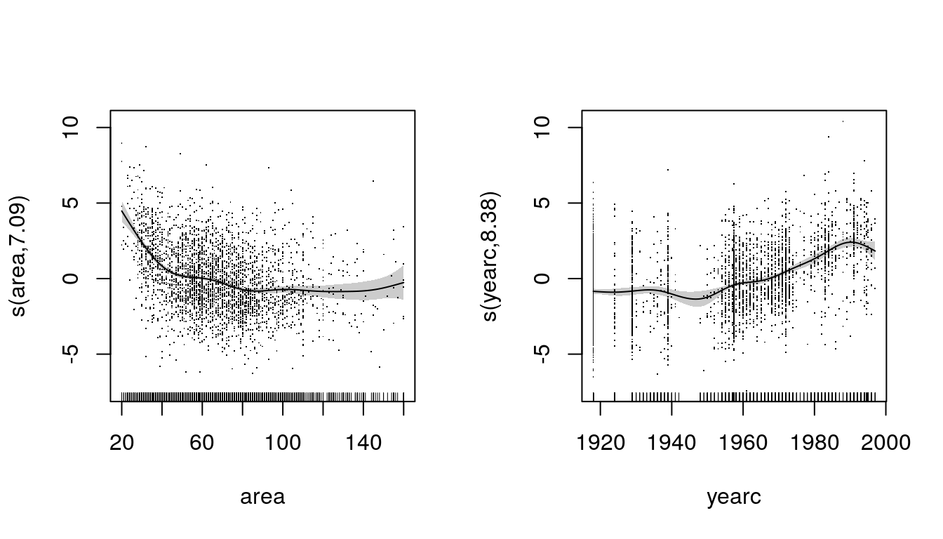
The label on the y-axis also reports the estimated degrees of freedom that are used to fit the smooth function. In addition, a summary method for the returned fitted model object exists
summary(b)##
## Family: gaussian
## Link function: identity
##
## Formula:
## rentsqm ~ s(area) + s(yearc)
##
## Parametric coefficients:
## Estimate Std. Error t value Pr(>|t|)
## (Intercept) 7.11126 0.03648 195 <2e-16 ***
## ---
## Signif. codes: 0 '***' 0.001 '**' 0.01 '*' 0.05 '.' 0.1 ' ' 1
##
## Approximate significance of smooth terms:
## edf Ref.df F p-value
## s(area) 7.094 8.061 72.26 <2e-16 ***
## s(yearc) 8.381 8.876 78.17 <2e-16 ***
## ---
## Signif. codes: 0 '***' 0.001 '**' 0.01 '*' 0.05 '.' 0.1 ' ' 1
##
## R-sq.(adj) = 0.309 Deviance explained = 31.2%
## GCV = 4.1226 Scale est. = 4.1006 n = 3082Next to the linear model output (parameter "(Intercept)"), for each smooth term approximate
P-values are reported along with the estimated degrees of freedom. Note that the default
number of basis functions when calling s() is 10. However, due to the centering constraint
one basis function is dropped, such that the maximum degrees of freedom of a univariate smooth
term is 9 (we will introduce multivariate smooth terms later in the script). Hence, if the
summary statistic reports a value of the degrees of freedom close to the maximum possible,
this is an indication that we should increase the number of basis functions, in order to
capture more information. In this example we could increase both model terms to
## Model formula.
f <- rentsqm ~ s(area, k = 40) + s(yearc,k = 40)

## Estimate model.
b <- gam(f, data = MunichRent)

## Summary output.
summary(b)
##
## Family: gaussian
## Link function: identity
##
## Formula:
## rentsqm ~ s(area, k = 40) + s(yearc, k = 40)
##
## Parametric coefficients:
## Estimate Std. Error t value Pr(>|t|)
## (Intercept) 7.11126 0.03648 194.9 <2e-16 ***
## ---
## Signif. codes: 0 '***' 0.001 '**' 0.01 '*' 0.05 '.' 0.1 ' ' 1
##
## Approximate significance of smooth terms:
## edf Ref.df F p-value
## s(area) 8.088 10.13 57.18 <2e-16 ***
## s(yearc) 9.310 11.38 60.79 <2e-16 ***
## ---
## Signif. codes: 0 '***' 0.001 '**' 0.01 '*' 0.05 '.' 0.1 ' ' 1
##
## R-sq.(adj) = 0.309 Deviance explained = 31.3%
## GCV = 4.1262 Scale est. = 4.1015 n = 3082## Plot.
par(mfrow = c(1, 2))
plot(b, residuals = TRUE, scheme = 1)
Note that the estimated degrees of freedom did not change that much in this example, just the
effect of yearc deserves a little bit of extra freedom, but visually there seems to be no
difference.
The effect plots are very helpful, since we can immediately see if a covariate is important or not (besides the reported P-values). For example, if an effect is not significant the effect plot will show a function that is basically following the zero horizontal line. In general, it is always a good idea to have a look at the 95% credible intervals. If these cover most of the time the zero horizontal line the effect is most probably not significant.
Moreover, per default the y-axis of the effect plots are scaled the same, this can be switched
of setting argument scale = 0 in the plotting function. By setting the same scale we can
immediately judge the importance of the effects, i.e., the more important the effect the larger
will be the absolute difference from the minimum to the maximum of the effect on the y-axis.
Predictions can be obtained in the same as for function lm(). However, if interested
in predictions for the single smooth terms, these can be obtained bay setting argument
type = "terms" in the predict method.
p <- predict(b, type = "terms")
print(head(p))
## s(area) s(yearc)
## 1 1.52920799 -0.9368259
## 2 -0.74412755 -0.9368259
## 3 2.57813291 0.3580268
## 4 0.96794902 0.4548525
## 5 -0.73818514 1.9548858
## 6 -0.03445875 -0.2598159Note that this call returns a matrix of the centered effects. For more details please see
?predict.gam.