Chapter 1 Linear regression

1.1 Model definition

Before we can really start dealing with flexible regression we should take a closer look at the linear regression model.

Recall the linear regression model, for \(i = 1, \dots, n\) observations, the model is defined by \[\begin{eqnarray*} y_i &=& f(x_{i1}, \dots, x_{ik}) + \varepsilon_i \\ &=& \beta_0 + \beta_1 x_{i1} + \ldots + \beta_k x_{ik} + \varepsilon_i \\ &=& \beta_0 + \sum_{j = 1}^k \beta_j x_{ij} + \varepsilon_i \\ &=& \mathbf{x}_i^\top\boldsymbol{\beta} + \varepsilon_i. \end{eqnarray*}\] In matrix notation this can be written as \[ \mathbf{y} = \mathbf{X}\boldsymbol{\beta} + \boldsymbol{\varepsilon}, \] with errors \(\boldsymbol{\varepsilon} \sim N(\mathbf{0}, \sigma^2\mathbf{I})\). Here, the matrix \(\mathbf{X}\) is the so called design matrix, or regressor matrix. Note, if the model has an intercept the first column of \(\mathbf{X}\) is a column of ones.

The aim is to estimate the unknown function \(f( \cdot )\), i.e., to separate the systematic component \(f( \cdot )\) from the random noise \(\boldsymbol{\varepsilon}\).

1.2 Parameter estimation

Least squares

Estimation of the linear model is done via least-squares optimization. \[ LS(\boldsymbol{\beta}) = \sum_{i = 1}^n\left(y_i - \mathbf{x}_i^\top\boldsymbol{\beta}\right)^2 = \boldsymbol{\varepsilon}^\top\boldsymbol{\varepsilon}. \] In matrix notation we get \[ \mathbf{X} = \begin{pmatrix} 1 & x_{11} & \cdots & x_{1k} \\ 1 & x_{21} & \cdots & x_{2k} \\ \vdots & \vdots & & \vdots \\ 1 & x_{n1} & \cdots & x_{nk} \end{pmatrix} \quad \boldsymbol{\beta} = \begin{pmatrix} \beta_0 \\ \beta_1 \\ \vdots \\ \beta_k \end{pmatrix} \quad \boldsymbol{\eta} = \mathbf{X}\boldsymbol{\beta}. \] Minimize \(||\mathbf{y} - f(\mathbf{x}_1, \ldots, \mathbf{x}_k)||^2 = ||\mathbf{y} - \boldsymbol{\eta}||^2 = ||\mathbf{y} - \mathbf{X}\boldsymbol{\beta}||^2\).

In order to determine the minimum of \(LS(\boldsymbol{\beta})\), we rearrange and obtain \[\begin{align} LS(\boldsymbol{\beta}) &= \boldsymbol{\varepsilon}^\top\boldsymbol{\varepsilon} \\ &= (\mathbf{y} - \mathbf{X} \boldsymbol{\beta})^\top(\mathbf{y} - \mathbf{X} \boldsymbol{\beta}) \\ &= \mathbf{y}^\top\mathbf{y} - \boldsymbol{\beta}^\top \mathbf{X}^\top \mathbf{y} - \mathbf{y}^\top \mathbf{X} \boldsymbol{\beta} + \boldsymbol{\beta}^\top \mathbf{X}^\top \mathbf{X} \boldsymbol{\beta} \\ &= \mathbf{y}^\top \mathbf{y} - 2 \, \mathbf{y}^\top \mathbf{X} \boldsymbol{\beta} + \boldsymbol{\beta}^\top\mathbf{X}^\top \mathbf{X} \boldsymbol{\beta}. \end{align}\] Note that \(\boldsymbol{\beta}^\top\mathbf{X}^\top\mathbf{y}\) and \(\mathbf{y}^\top\mathbf{X}\boldsymbol{\beta}\) (as well as \(\mathbf{y}^\top\mathbf{y}\) and \(\boldsymbol{\beta}^\top\mathbf{X}^\top\mathbf{X}\boldsymbol{\beta}\)) are scalars. Thus \(\boldsymbol{\beta}^\top\mathbf{X}^\top\mathbf{y} = (\boldsymbol{\beta}^\top\mathbf{X}^\top\mathbf{y})^\top = \mathbf{y}^\top\mathbf{X}\boldsymbol{\beta}\). \[\begin{align} \frac{\partial LS(\boldsymbol{\beta})}{\partial \boldsymbol{\beta}} &= -2\mathbf{X}^\top\mathbf{y} + 2\mathbf{X}^\top\mathbf{X}\boldsymbol{\beta} = \mathbf{0} \\ &\Rightarrow \hat{\boldsymbol{\beta}} = (\mathbf{X}^\top\mathbf{X})^{-1}\mathbf{X}^\top\mathbf{y} \\ &\Rightarrow \hat{\mathbf{y}} = \mathbf{H}\mathbf{y} = \mathbf{X}(\mathbf{X}^\top\mathbf{X})^{-1}\mathbf{X}^\top\mathbf{y} \end{align}\]

Here, \(\mathbf{H}\) is the so called hat-matrix, a matrix that maps the response observations to the fitted regression plane. This matrix will be important for the estimation of general smooth functions. Properties of the hat-matrix:

\(\mathbf{H}\) is symmetric.
\(\mathbf{H}\) is idempotent.
\(rk(\mathbf{H}) = tr(\mathbf{H}) = p\), i.e., the trace is equal to the rank and \(p\) is the number of parameters in the model.
\(\frac{1}{n}\leq h_{ii}\leq \frac{1}{r}\), where \(r\) represents the number of rows in \(\mathbf{X}\) with different \(\mathbf{x}_i\). If the rows are all different, then \(\frac{1}{n}\leq h_{ii}\leq 1\).
The matrix \(\mathbf{I} - \mathbf{H}\) is also symmetric and idempotent, with \(rk(\mathbf{I}-\mathbf{H}) = n - p\).

Maximum likelihood

Assuming normally distributed errors, i.e., \(\boldsymbol{\varepsilon} \sim N(\mathbf{0}, \sigma^2\mathbf{I})\), the maximum likelihood (ML) estimator for the unknown parameters can be computed with \[ L(\boldsymbol{\beta}, \sigma^2) = \frac{1}{\left( 2\pi\sigma^2 \right)^{n \!/ 2}} \exp \left( -\frac{1}{2 \sigma^2} (\mathbf{y} - \mathbf{X} \boldsymbol{\beta})^\top(\mathbf{y} - \mathbf{X}\boldsymbol{\beta}) \right), \] and \[ \ell(\boldsymbol{\beta}, \sigma^2) = -\frac{n}{2}\log(2\pi) - \frac{n}{2}\log(\sigma^2) - \frac{1}{2 \sigma^2} (\mathbf{y} - \mathbf{X} \boldsymbol{\beta})^\top(\mathbf{y} - \mathbf{X}\boldsymbol{\beta}). \] Hence \[ \Rightarrow \,\, \hat{\boldsymbol{\beta}} = (\mathbf{X}^\top\mathbf{X})^{-1}\mathbf{X}^\top\mathbf{y}. \]

Differentiation of the log-likelihood with respect to \(\sigma^2\), and setting to zero \[ \frac{\partial \ell(\boldsymbol{\beta},\sigma^2)}{\partial \sigma^2} = - \frac{n}{2\sigma^2} + \frac{1}{2\sigma^4}(\mathbf{y} - \mathbf{X}\boldsymbol{\beta})^\top( \mathbf{y} - \mathbf{X} \boldsymbol{\beta} ) \stackrel{!}{=} 0. \] Substituting the ML or least squares estimator \(\hat{\boldsymbol{\beta}}\) \[ -\frac{n}{2\sigma^2}+\frac{1}{2 \sigma^4} (\mathbf{y} - \hat{\mathbf{y}})^\top (\mathbf{y} - \hat{\mathbf{y}}) = -\frac{n}{2 \sigma^2}+\frac{1}{2 \sigma^4} \hat{\boldsymbol{\varepsilon}}^\top \hat{\boldsymbol{\varepsilon}} \stackrel{!}{=} 0, \] yielding \[ \hat{\sigma}_{ML}^2 = \frac{\hat{\boldsymbol{\varepsilon}}^\top \hat{\boldsymbol{\varepsilon}}}{n}. \]

However, this estimator for \(\sigma^2\) is rarely used. The mean of the sum of squared residuals is \[ E(\hat{\boldsymbol{\varepsilon}}^\top\hat{\boldsymbol{\varepsilon}}) = (n - p) \cdot \sigma^2, \] and thus \[ E(\hat{\sigma}^2_{ML}) = \frac{n - p}{n} \sigma^2. \] Hence, the ML estimator for \(\sigma^2\) is biased. An unbiased estimator is \[ \hat{\sigma}^2 = \frac{1}{n - p} \hat{\boldsymbol{\varepsilon}}^\top\hat{\boldsymbol{\varepsilon}}. \]

Estimation in R

Linear models can be estimated using the lm() function, see ?lm for details as well as the upcoming examples.

Goodness-of-fit

To provide a first tool to judge the goodness-of-fit of an estimated regression model we can look at the corrected coefficient of determination (adjusted \(R^2\)), which is given by \[ \bar{R}^2 = 1-\frac{n - 1}{n - p}(1 - R^2). \] where \[ R^2 = 1 - \frac{SS_{res}}{SS_{tot}} \] and \(SS_{res}\) is the residuals sum of squares and \(SS_{tot}\) is the total sum of squares. Hence, this measure provides insight on how much percent of the total variation in the data can be explained by the model. The adjusted \(R^2\) penalizes for the complexity of the model, i.e., the number of parameters and therefore tries to minimize the out-of-sample error in some way.

The adjusted \(R^2\) can be extracted using the summary() method after fitting a linear model with lm() (see also the examples).

More details on goodness-of-fit criteria will be presented in the upcoming chapters.

1.3 Assumptions

Of course, the model has some assumptions on which it is based, and if these are not fulfilled, problems can sometimes arise in the approximation of \(f( \cdot )\), moreover, hypothesis tests on the unknown parameters \(\boldsymbol{\beta}\) are not valid and can lead to wrong interpretations of the covariate effects. The following list gives an overview of the most important assumptions:

The systematic component \(f( \cdot )\) is a linear combination of covariates.
Additive errors \(\boldsymbol{\varepsilon}\).
Expectation of the errors, \(E(\boldsymbol{\varepsilon}) = \mathbf{0}\).
Variances and correlation structure of the errors, constant error variance \(\sigma^2\) across observations, uncorrelated errors, resulting covariance matrix \(Cov(\boldsymbol{\varepsilon}) = E(\boldsymbol{\varepsilon}\boldsymbol{\varepsilon}^\top) = \sigma^2\mathbf{I}\).
Assumptions about the covariates and the design matrix, \(E(\boldsymbol{\varepsilon} | \mathbf{X}) = \mathbf{0}\), \(Cov(\boldsymbol{\varepsilon} | \mathbf{X}) = \sigma^2\mathbf{I}\). However, the assumption that errors and stochastic covariates are independent can be relaxed \(Var(\varepsilon_i | \mathbf{x}_i) = \sigma^2(\mathbf{x}_i)\).
Gaussian errors, \(\boldsymbol{\varepsilon} \sim N(\mathbf{0}, \sigma^2\mathbf{I})\).

From our model assumptions it immediately follows that \[ \begin{array}{rll} E(y_i) & = & E(\mathbf{x}_i^\top \boldsymbol{\beta} + \varepsilon_i) = \mathbf{x}_i^\top \boldsymbol{\beta} = \beta_{0} + \beta_{1} x_{i1} + \ldots + \beta_{k} x_{ik}, \\[0.2cm] Var(y_i) & = & Var(\mathbf{x}_i^\top \boldsymbol{\beta} + \varepsilon_i) = Var(\varepsilon_i) = \sigma^2, \\[0.2cm] Cov(y_i,y_j) & = & Cov(\varepsilon_i,\varepsilon_j) = 0, \end{array} \] for the mean and the variance of \(y_i\), as well as the covariance between \(y_i\) and \(y_j\). In matrix notation \[ E(\mathbf{y}) = \mathbf{X} \boldsymbol{\beta} \quad \mbox{and} \quad Cov(\mathbf{y}) = \sigma^2 \mathbf{I}. \] Assuming normally distributed errors, we have \[ \mathbf{y} \sim N(\mathbf{X} \boldsymbol{\beta},\sigma^2 \mathbf{I}). \] Hence, for each observation a normal distribution with mean \(\mathbf{x}_i^\top \boldsymbol{\beta}\) is assigned and the variance \(\sigma^2\) is assumed to be constant for all observations \(i = 1, \ldots, n\), homoskedastic.

Let’s illustrate this using some simulated data with \[ y_i = 2 + 1.5 \cdot x_i + \varepsilon_i, \qquad i = 1, \ldots, 100, \] where the error is \(\varepsilon_i \sim N(0, 0.2^2)\) and \(x_i \sim U(0,1)\):

## Set the seed for reproducibility.
set.seed(123)

## Simulate data.
n <- 100
x <- runif(n)
y <- 2 + 1.5 * x + rnorm(n, sd = 0.2)

## Scatterplot.
par(mar = c(4.1, 4.1, 0.1, 0.1))
plot(x, y)

## Estimate linear model and add the fitted line
## to the scatterplot.
b <- lm(y ~ x)
abline(b)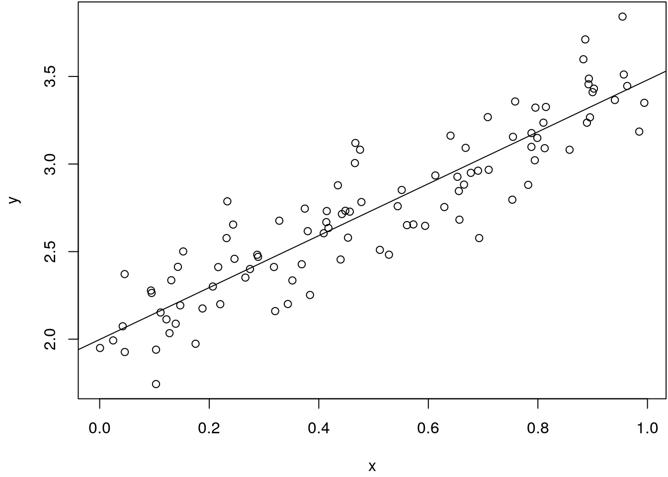

The estimated standard deviation can be extracted with

(sdb <- summary(b)$sigma)

## [1] 0.1938582

which is almost the true value of \(0.2\) we used to simulate the data. We can use this estimate to illustrate the constant variance assumption by adding estimated conditional densities to our figure. This is a bit technical:

## Function to draw a vertical normal density.
vert_dens <- function(x, y, sd = 0.2, height = 0.05) {
  xlim <- par()$usr[1:2]
  ylim <- par()$usr[3:4]
  xp <- seq(ylim[1], ylim[2], length = 100)
  d <- dnorm(xp, mean = y, sd = sd)
  d <- d / diff(range(d)) * height
  x <- rep(x, length.out = length(xp))
  col <- gray(0.9)
  polygon(c(x + d, rev(x)), c(xp, rev(xp)),
    border = NA, col = col)
  lines(x + d, xp)
}

## New data for plotting.
nd <- data.frame("x" = rev(seq(0.1, 0.9, length = 20)))
nd$p <- predict(b, newdata = nd)

## Add density to plot
par(mar = c(4.1, 4.1, 0.1, 0.1))
plot(x, y)
abline(b)
for(i in 1:nrow(nd))
  vert_dens(nd$x[i], nd$p[i], sd = sdb)
points(x, y)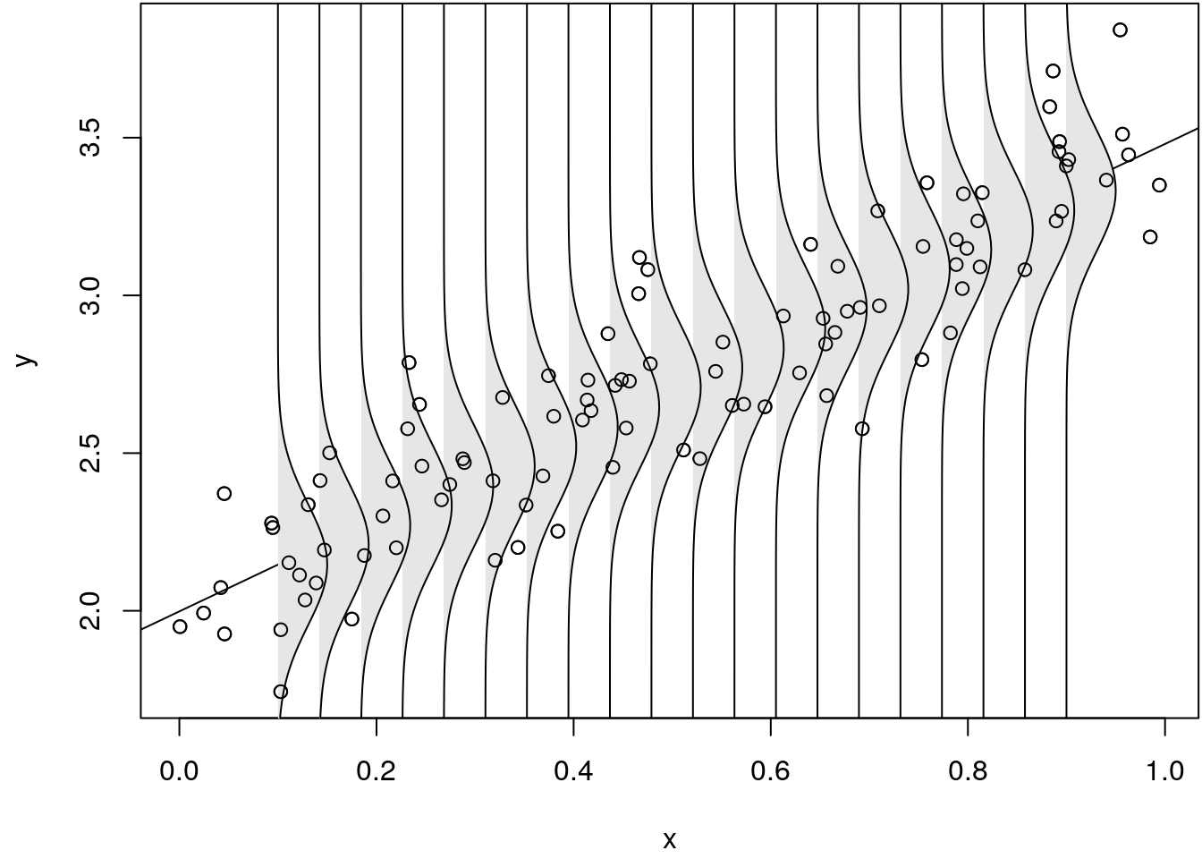

This figure illustrates, that for each observation \(i\) a normal distribution with mean \(\mathbf{x}_i^\top\boldsymbol{\beta}\) is fitted to the data. Instead of plotting the estimated conditional normal densities, we could also simply highlight the areas of high probability.

## Function to draw conditional densities as image.
img_dens <- function(object) {
  xlim <- par()$usr[1:2]
  ylim <- par()$usr[3:4]
  yp <- seq(ylim[1], ylim[2], length = 100)
  xp <- seq(xlim[1], xlim[2], length = 100)
  xm <- xp[-100] + diff(xp[1:2]) / 2
  ym <- yp[-100] + diff(yp[1:2]) / 2
  sd <- summary(object)$sigma
  p <- predict(object, newdata = data.frame("x" = xm))
  d <- matrix(NA, 99, 99)
  for(i in 1:99) {
    d[i, ] <- dnorm(ym, mean = p[i], sd = sd)
  }
  image(xm, ym, d, add = TRUE, col = rev(colorspace::heat_hcl(99)))
}

## Add density to plot
par(mar = c(4.1, 4.1, 0.1, 0.1))
plot(x, y)
img_dens(b)
abline(b)
points(x, y)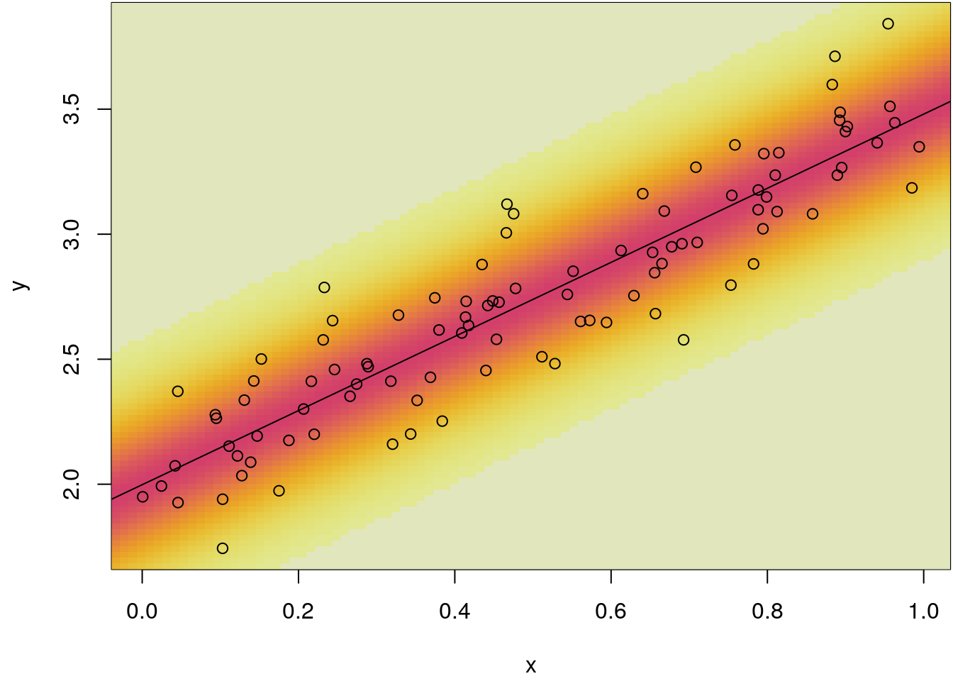

So if the constant variance assumption is violated, inference for example for new data points can be problematic. This is illustrated in the following practical simulated example.

Exercise 1.1 Simulate heteroskedastic data with \[ y_i = 2 + 1.5 \cdot x_i + \varepsilon_i \cdot \exp(-2 + 4 \cdot x_i), \qquad i = 1, \ldots, 100, \] with \(x_i \sim U(0, 1)\). Estimate a linear model in the same fashion as in the example above. Visualize the predictive distribution with function img_dens(). Interpret the results.

The data can be simulated with

## Set the seed for reproducibility.
set.seed(456)

## Simulate heteroskedastic data.
n <- 100
x <- runif(n)
y <- 2 + 1.5 * x + rnorm(n, sd = 0.2) * exp(-2 + 4 * x)

The linear model is then estimated as shown in the above. Also the predictive distribution is visualized accordingly.

## Estimate linear model.
b <- lm(y ~ x)

## Estimates standard deviation
summary(b)$sigma

## [1] 0.5916208

## Scatterplot with density estimates.
par(mar = c(4.1, 4.1, 0.1, 0.1))
plot(x, y)
img_dens(b)
abline(b)
points(x, y)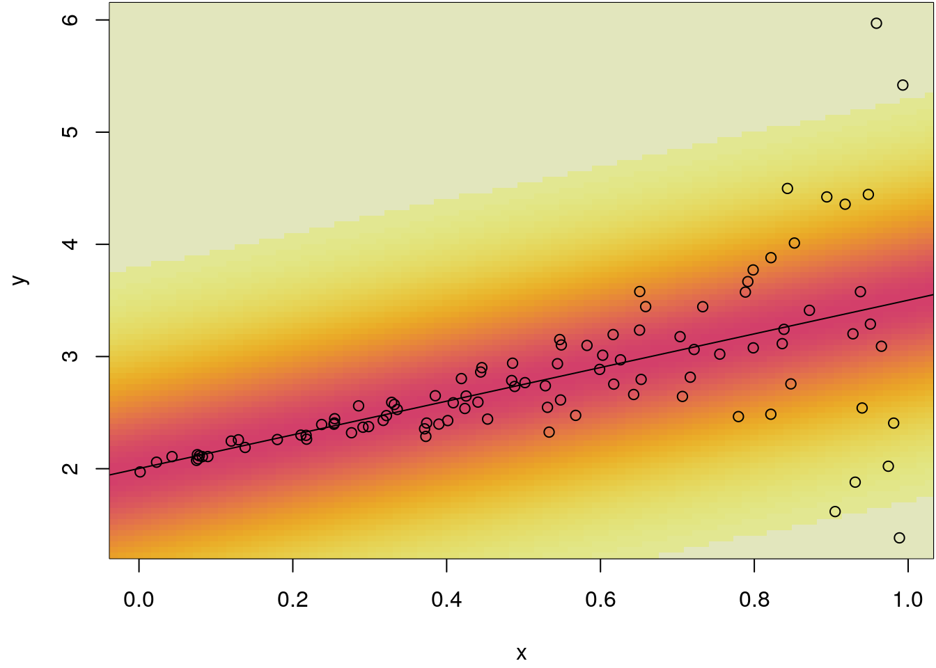

The plot clearly shows that the predictive distribution has too wide tails for small values of the covariate x, this is caused by the homoskedasticity assumption with estimated global standard deviation of 0.59.

1.4 Discussion of assumptions

At first glance, the linear model may seem a little inflexible, or the assumptions rather restrictive. In the following we show that, e.g., the assumption of linearity is not as daunting as one might assume. Sometimes many resulting problems in the linear model can easily be solved by transformations of covariates and the response.

Linearity

It may not be quite obvious at first glance, but nonlinear relationships can also be modelled. In the simplest case a nonlinear function can be estimated by a simple transformation of the covariates. Why is this possible? In order to better explain the effect, we would like to introduce the concept of basis functions at this point. In the simple linear model a basic function is given as \[ y = \beta_0 + B(x_i) \cdot \beta_1 + \varepsilon_i = \beta_0 + x_i \cdot \beta_1 + \varepsilon_i, \] hence the used basis function is simply the identity function with \(B(x_i) = x_i\). Technically what happens is that we scale the basis function \(B(x_i)\) with the corresponding regression coefficient \(\beta_1\) such that we best approximate the relationship between \(x\) and \(y\). This is illustrated in the following simulated example:

## Set the seed for reproducibility.
set.seed(123)

## Simulate data.
n <- 100
x <- runif(n)
y <- 2 + 1.5 * x + rnorm(n, sd = 0.2)

## Scatterplot.
par(mar = c(4.1, 4.1, 0.1, 0.1))
plot(x, y)

## Estimate linear model.
b <- lm(y ~ x)

## Extract coefficients.
cb <- coef(b)

## Draw unscaled basis function to scatterplot.
i <- order(x)
fit0 <- cb["(Intercept)"] + x[i]
lines(fit0 ~ x[i], col = 1, lwd = 2)

## Add scaled basis function.
i <- order(x)
fit1 <- cb["(Intercept)"] + cb["x"] * x[i]
lines(fit1 ~ x[i], col = 2, lwd = 2)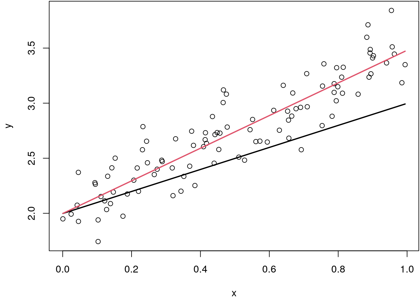

Here, the black line represents the unscaled basis, the red line is the scaled basis function which perfectly fits through the data.

This concept is very useful for estimating nonlinear relationships since we can use any type of basis function \(B( \cdot )\), e.g., a logarithmic nonlinear effect of explanatory variable \(x_i\) can be obtained by \[ y_i = \beta_0 + \beta_1 B(z_i) + \varepsilon_i = \beta_0 + \beta_1 \log(x_i) + \varepsilon_i. \] In general, nonlinear relationships can be connected to linear models provided that they are linear in the parameters.

The following is an example for a model, which is nonlinear in the parameter \(\beta_2\) is given by \[ y_i = \beta_0 + \beta_1 \sin(\beta_2 x_i) + \varepsilon_i. \] This model can also be estimated from the data, however, th estimation algorithm is slightly a bit more complicated as for the linear regression model.

Exercise 1.2 Use the MunichRent data and estimate the following linear model \[ \texttt{rentsqm}_i = \beta_0 + B(\texttt{area}_i) \cdot \beta_1 + \varepsilon_i. \] For the basis function \(B( \cdot )\) use the identity, logarithmic, inverse and square root transformation function. Which transformation approximates the relationship best?

First, we load the data

load("data/MunichRent.rda")

The three models can be estimated with

b1 <- lm(rentsqm ~ area, data = MunichRent)
b2 <- lm(rentsqm ~ log(area), data = MunichRent)
b3 <- lm(rentsqm ~ I(1/area), data = MunichRent)
b4 <- lm(rentsqm ~ sqrt(area), data = MunichRent)

For the moment, the best way to judge which model fits best to the data we compare by drawing the fitted lines in the scatterplot.

p1 <- predict(b1)
p2 <- predict(b2)
p3 <- predict(b3)
p4 <- predict(b4)

par(mar = c(4.1, 4.1, 0.1, 0.1))
plot(rentsqm ~ area, data = MunichRent, col = rgb(0.1, 0.1, 0.1, alpha = 0.4))
i <- order(MunichRent$area)
lines(p1[i] ~ MunichRent$area[i], col = 2, lwd = 2)
lines(p2[i] ~ MunichRent$area[i], col = 3, lwd = 2)
lines(p3[i] ~ MunichRent$area[i], col = 4, lwd = 2)
lines(p4[i] ~ MunichRent$area[i], col = 5, lwd = 2)
legend("topright", c("identity", "logarithmic", "inverse", "square root"),
  lwd = 2, col = 2:5)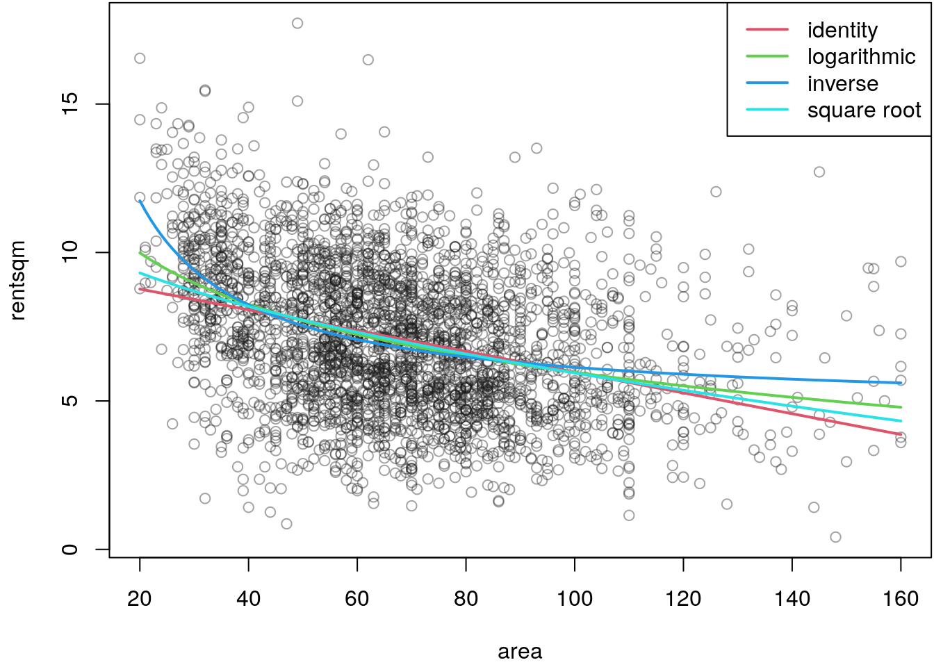

The plot suggests that the inverse transformation function seems to approximate the dependence of rentsqm on the area of the apartment best, since there the strong decrease of prices for very small apartments is most plausible. Note that this judgment only relies on graphical inspection, in the upcoming we will learn how to choose models more automatically.

Uncorrelated errors

In the exercise with the heteroskedastic errors in section Assumptions, we have already learned that problems can occur, i.e., according to the predictive distribution, if the error variance is non-constant. Similar problems arise if the errors are correlated, i.e., again the assumption of independent and identically distributed (i.i.d.) errors is violated. Especially in time series and longitudinal data, the assumption of uncorrelated errors is not realistic. Just imagine the price of the Google stock:

## Warning: `type_convert()` only converts columns of type 'character'.
## - `df` has no columns of type 'character'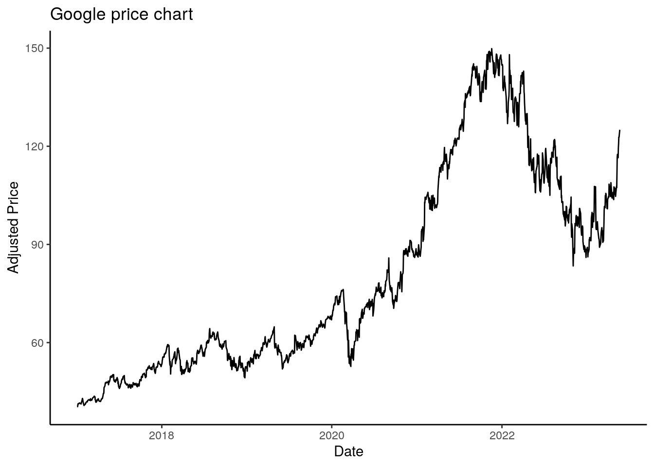

The plot clearly shows that the price of today is dependent on yesterdays prices, so these are definitely correlated.

The time-series structure of the data is a topic itself, so if we do not account for this, inference about the model parameters is critical. However, problems with correlated errors can also occur if we simply miss-specify the underlying functional relationship. In the example with the Munich rent index from section Linearity, we already played a bit with the correct non-linear functional form. To see that a wrongly chosen representation of the functional form can lead to correlated errors, let’s again have a look at a simulated data example:

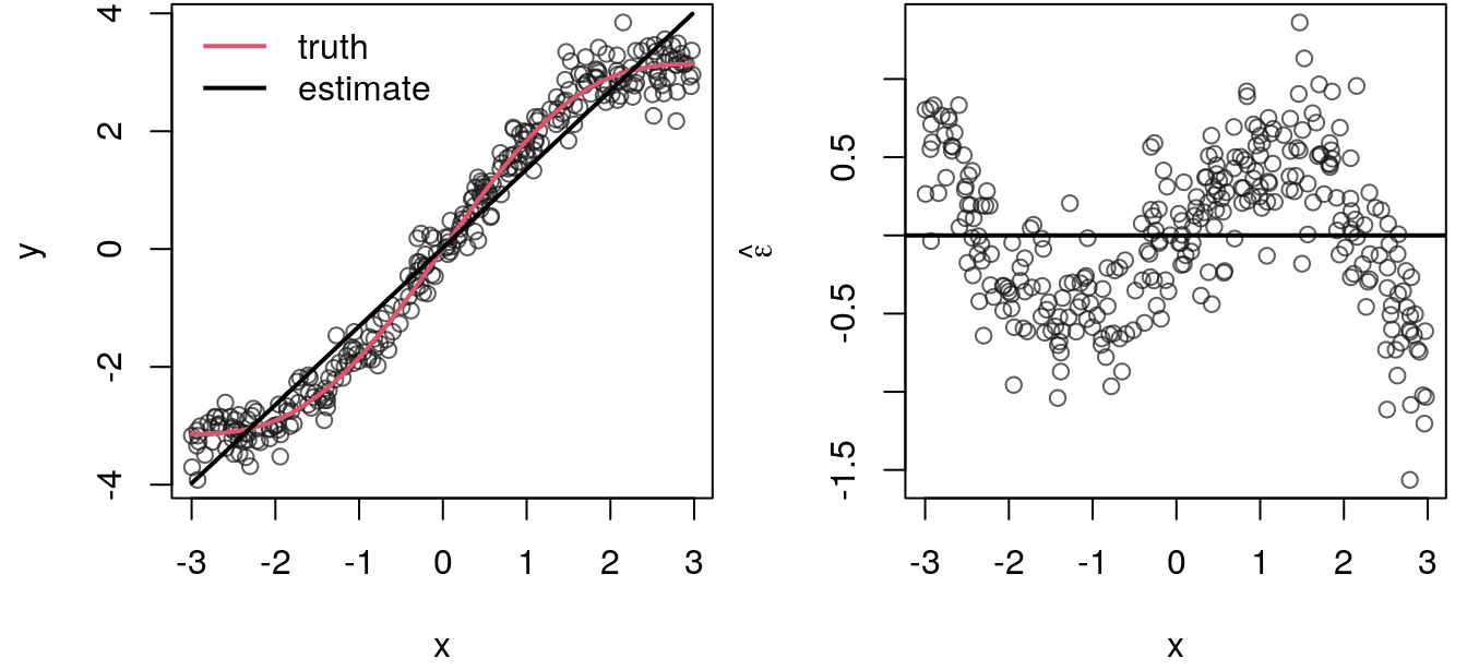
The plot shows a slightly nonlinear function as the true data generating process. Now, if we estimate a linear model, the straight line will surely not model the full signal, hence, if we look to the right panel of the resulting residuals, we can see that there is quite a lot of correlation. Either the residuals lie above or below the zero horizontal line instead of fluctuation like random (white) noise.

Time trends in covariates

The problem of autocorrelation in the residuals can not only arise from a misspecification of the functional relationship, but also, for example, if we forget to include an important covariable that follows a temporal trend in the model. This is illustrated in the following graphic:

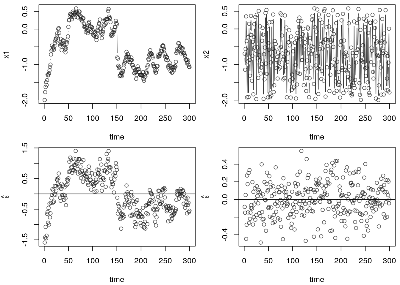
The upper left panel shows the values of covraite x1 over time. We can clearly see that the variable has a quite strong time trend. The second covariate x2 is shown in the upper right panel. Here, the value fluctuate unstructured over time. Now, we simulate data with \[ y_i = 2 + x_{1i} - x_{2i} + \varepsilon_i, \] with \(\varepsilon_i \sim N(0, 0.2^2)\) and estimate two models: (1) a model without the time-trend covariate x1 and a model including it. Then we can see in the lower left panel, that the residuals have a very strong time pattern, i.e., have a strong correlation. If instead, we estimate the correct model including both variables x1 and x2, the residuals shown in the lower right panel show i.i.d. behavior. So missing out important variables that follow a time-trend can be quite critical.

Additive errors

In principle, many different models for the structure of the errors are conceivable. In the vast majority of cases, two alternative error structures are assumed: additive errors and multiplicative errors.

Example: exponential model \[ \begin{array}{lll} y_i & = & \exp(\beta_0 + \beta_1 x_{i1} + \ldots + \beta_k x_{ik} + \varepsilon_i) \\[0.2cm] & = & \exp(\beta_0) \exp(\beta_1 x_{i1}) \cdot \ldots \cdot \exp(\beta_k x_{ik}) \exp(\varepsilon_i). \\ \end{array} \] with multiplicative errors \(\tilde \varepsilon_i = \exp(\varepsilon_i)\).

However, a logarithmic transformation results in the linear model \[ \log(y_i) = \beta_0 + \beta_1 x_{i1} + \ldots + \beta_k x_{ik} + \varepsilon_i. \]

Log-normal distributed responses.

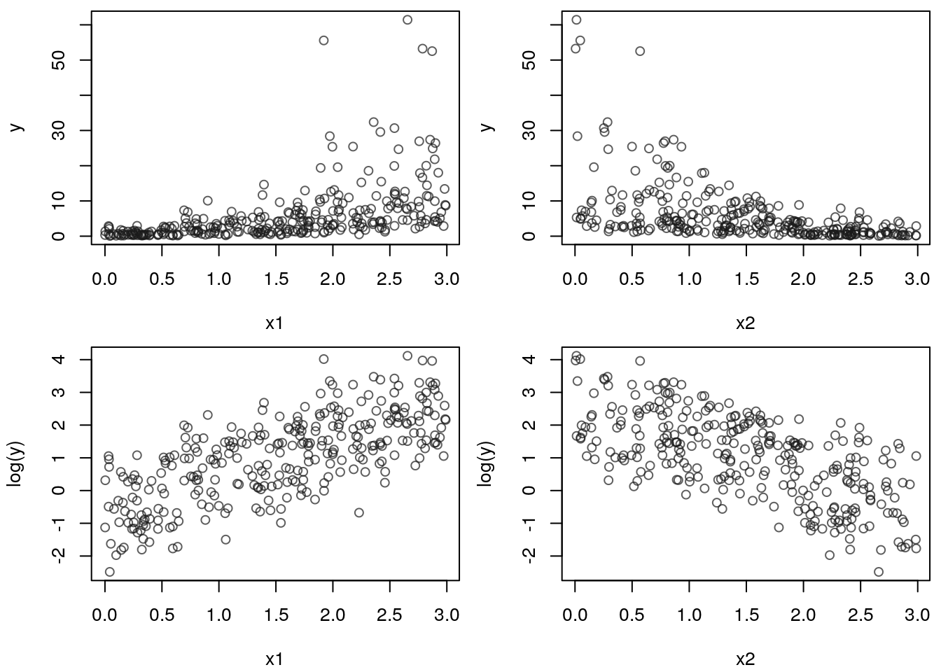
Here, we again simulated data with two covariates, but with an exponential structure \[ y_i = \exp(1 + x_{1i} - x_{2i} + \varepsilon_i), \] with \(\varepsilon_i \sim N(0, 0.4^2)\). The upper left plot shows the scatterplot of the simulated response y and covariate x1, the upper right panel the scatterplot of y and x2, respectively. Looking at the two panels it is hard to see the functional relationship. However, if we apply a logarithmic transformation of the response the relationship immediately becomes clearer. This is illustrated in the lower right and left panel. We can clearly see the linear increasing effect of covariate x1 and the linear decreasing effect of x2. Hence, with the help of a simple transformation of the response variable we again meet the model assumptions.

1.5 Modeling the effects of covariates

Using the Munich rent index data we specify the following model: \[ \texttt{rentsqm}_i = \beta_0 + \beta_1\texttt{area}_i + \varepsilon_i. \]

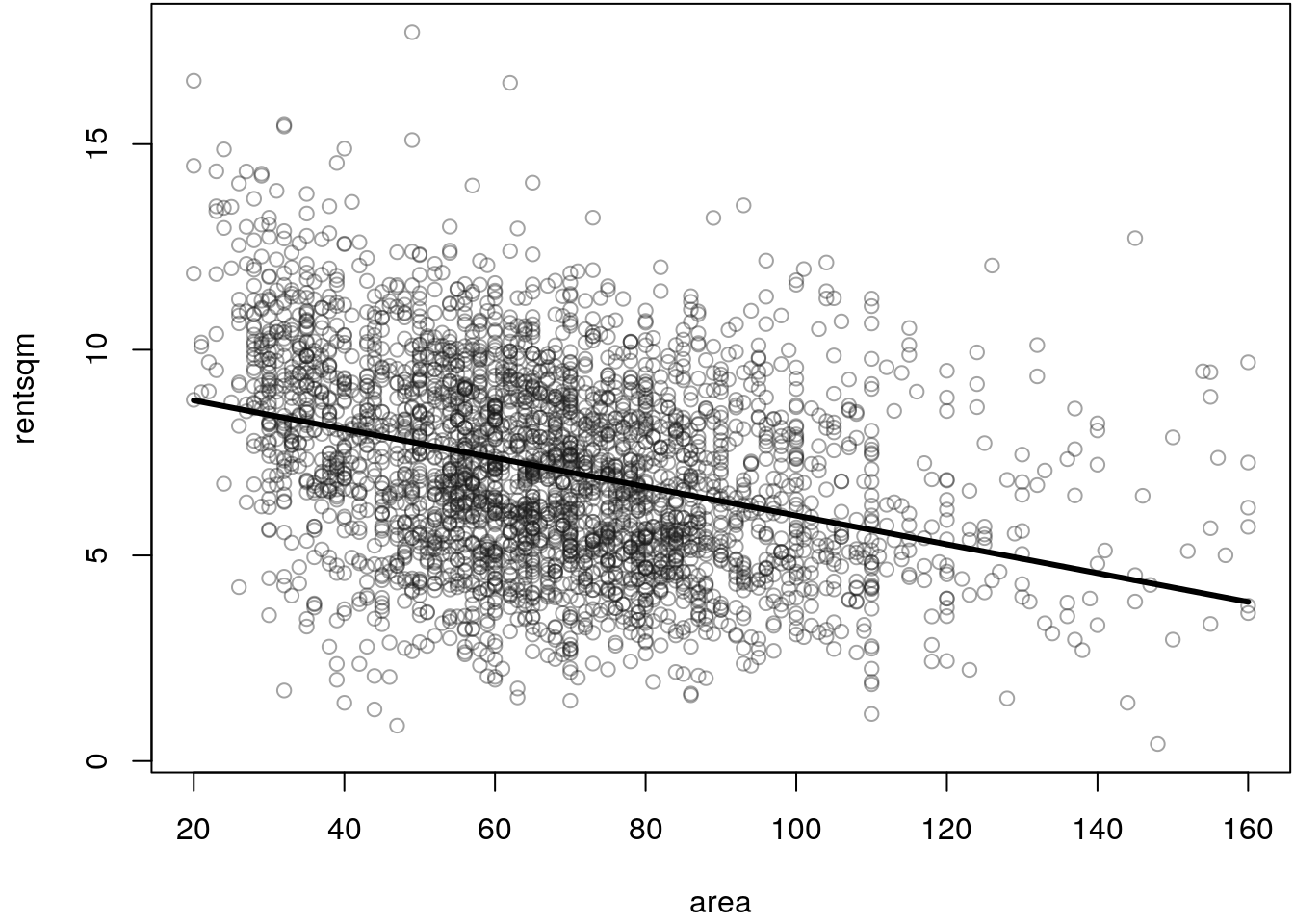
The residuals are mostly positive for smaller apartments (\(\texttt{area} < 30\)), indicating a nonlinear relationship.

Now consider the regression model \[ \texttt{rentsqm}_i = \beta_0 + B(\texttt{area}_i) \cdot \beta_1 + \varepsilon_i, \] where \(B( \cdot )\) is an arbitrary function. The function \(B( \cdot )\) must be appropriately specified, i.e., \(B( \cdot )\) itself is fixed in advance and not estimated. As we have seen before, this is a generalization of the linear model, i.e., this is a simple case of a basis function approach, where the basis function transformation function \(B( \cdot )\) can be of any type (e.g., logarithmic, square root, inverse, exponential, etc.).

Now, we can even further generalize the model and write \[ \texttt{rentsqm}_i = \beta_0 + B(\texttt{area}_i) \cdot \beta_1 + \varepsilon_i = \beta_0 + f_1(\texttt{area}_i) + \varepsilon_i, \] where function \(f_1( \cdot )\) can be any type of function, which needs to be estimated from the data. In the upcoming we will see that such functions can be really flexible, although its structure will again be linear in the parameters, so we can use the standard least squares estimator. Function \(f_1( \cdot )\) must not necessarily be a single transformation function, it can also be a complicated decomposition of transformation functions, as long as the problem is linear in the parameters. This is for example the case using polynomial regression, which is presented in the upcoming.

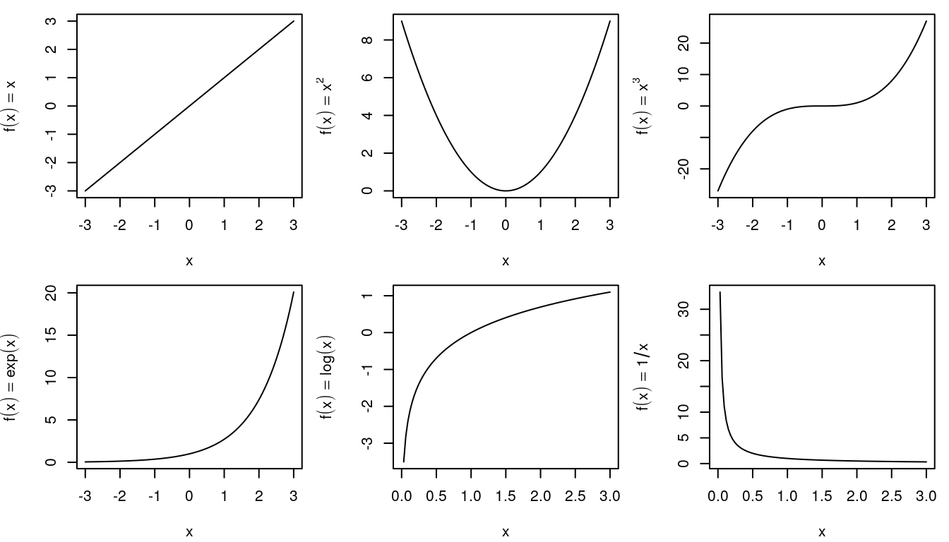
Standard transformations

As already mentioned, we can use transformation functions for the covariates, i.e., the basis function approach, and we can also transform the response variable such that the resulting model better follows the assumptions of the linear regression model. The following graphic illustrates commonly used transformations of covariates and response variables.

Exercise 1.3 Load the UsedCars data and estimate linear models with \[ Y(\texttt{price}_i) = \beta_0 + \beta_1 B(\texttt{age}_i) + \varepsilon_i, \] where functions \(Y( \cdot )\) and \(B( \cdot )\) can be any of the transformation functions presented in the above. Find the best fitting combination using the mean absolute percentage error (MAPE) of the re-transformed predicted values, i.e., the prices on the original scale.

The data is loaded with

load("data/UsedCars.rda")

Now, we estimate a series of linear models using the following transformations:

## Store all functions in a list.
trans_fun <- list("exp" = exp, "log" = log, "sqrt" = sqrt,
  "inverse" = function(x) { 1 / x }, "quadratic" = function(x) x^2)

## Get all combinations for Y() and B().
combos <- expand.grid(
  "Y" = names(trans_fun),
  "B" = names(trans_fun),
  stringsAsFactors = FALSE
)
print(combos)

##            Y         B
## 1        exp       exp
## 2        log       exp
## 3       sqrt       exp
## 4    inverse       exp
## 5  quadratic       exp
## 6        exp       log
## 7        log       log
## 8       sqrt       log
## 9    inverse       log
## 10 quadratic       log
## 11       exp      sqrt
## 12       log      sqrt
## 13      sqrt      sqrt
## 14   inverse      sqrt
## 15 quadratic      sqrt
## 16       exp   inverse
## 17       log   inverse
## 18      sqrt   inverse
## 19   inverse   inverse
## 20 quadratic   inverse
## 21       exp quadratic
## 22       log quadratic
## 23      sqrt quadratic
## 24   inverse quadratic
## 25 quadratic quadratic

## Function to compute the MAPE.
MAPE <- function(object, Y) {
  warn <- getOption("warn")
  options("warn" = -1)
  on.exit(options("warn" = warn))
  Yinv <- switch(Y,
    "exp" = log,
    "log" = exp,
    "sqrt" = function(x) x^2,
    "inverse" = function(x) { 1 / x },
    "quadratic" = sqrt
  )
  p <- Yinv(predict(object))
  y <- UsedCars$price
  mape <- mean(abs((p - y) / y), na.rm = TRUE)
  return(mape)
}

## Estimate models and extract the adjusted R-squared
## to find the best fitting combination.
mape <- rep(0, nrow(combos))
for(i in 1:nrow(combos)) {
  y <- trans_fun[[combos[i, "Y"]]](UsedCars$price)
  x <- trans_fun[[combos[i, "B"]]](UsedCars$age)
  b <- lm(y ~ x)
  mape[i] <- MAPE(b, combos[i, "Y"])
}

## Extract the best fitting combination.
i <- which.min(mape)
print(combos[i, ])

##          Y    B
## 14 inverse sqrt

## Reestimate model and plot.
y <- trans_fun[[combos[i, "Y"]]](UsedCars$price)
x <- trans_fun[[combos[i, "B"]]](UsedCars$age)
b <- lm(y ~ x)
par(mar = c(4.1, 4.1, 0.1, 0.1))
plot(y ~ x, xlab = "sqrt(age)", ylab = "1/price")
abline(b, lwd = 2)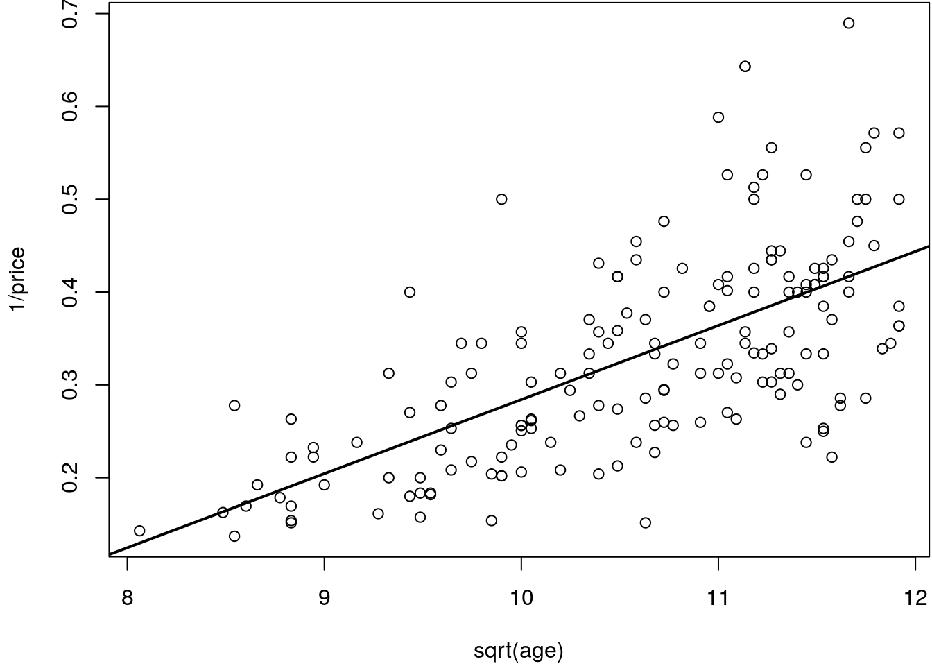

The figure indicates that the model fits quite well to the data, however, this plot is a bit difficult to interpret. We need to re-transform to the original scale to get a better impression of the relationship of the price and the age of the car.

## Predict on inverse scale.
p <- predict(b)

## Re-transform.
p <- 1 / p

## Plot again
par(mar = c(4.1, 4.1, 0.1, 0.1))
plot(price ~ age, data = UsedCars,
  ylim = range(c(UsedCars$price, p)))
i <- order(UsedCars$age)
lines(p[i] ~ age[i], data = UsedCars, lwd = 2)

The plot shows, that the relationship of price and age can be quite appropriately modeled using the inverse transformation for the dependent variable price and the square-root transformation for covariate age.

Polynomial regression

In many applications a simple transformation of the covariate can no longer be sufficient to get a satisfactory fit. A simple way to obtain more flexibility is to use polynomial regression \[ y_i = \beta_0 + x_i \beta_1 + x_i^2 \beta_2 + \ldots + x_i^l \beta_2 + \varepsilon_i. \] Typically, polynomials of a low degree \(l\) are preferred. In practice, we rarely use polynomials of degree higher than \(l = 3\), since the estimates can become quite unstable with high variability at the borders of the covariate domain. Moreover, numerical instabilities can arise for very high degrees, this is illustrated in the following simulated example.

## Set the seed for reproducibility.
set.seed(111)

## Simulate data.
n <- 100
## Sample very large values for x.
x <- runif(n, 1e+05, 1e+06)

## Simulate response data.
y <- 10 + x + 0.5 * x^2 + rnorm(n, sd = 1e+10)

## Show the scatterplot.
par(mar = c(4.1, 4.1, 0.1, 0.1))
plot(y ~ x)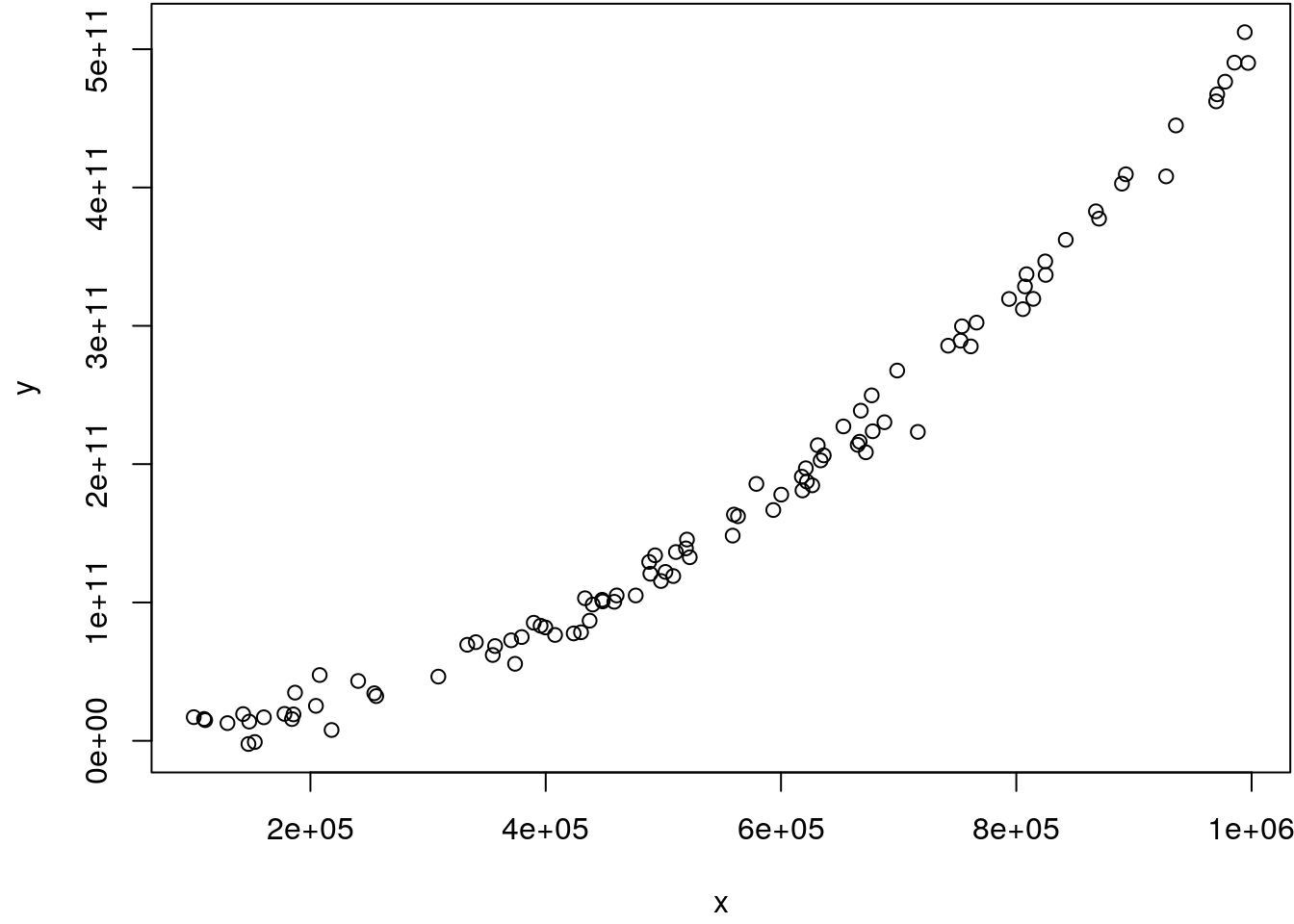

## Compute the design matrix.
X <- cbind(1, x, x^2)

## Estimate regression coefficients.
try(beta <- solve(crossprod(X)) %*% t(X) %*% y)

## Error in solve.default(crossprod(X)) : 
##   system is computationally singular: reciprocal condition number = 2.64875e-25

This gives an error. The reason for this is that the computer cannot represent any large number. Due to the quadratic transformation of the covariate, which already contains huge values, the calculation of the regression coefficients leads to a floating-point overflow, i.e. the inverse cannot be calculated anymore.

A solution is to scale the covariate values before applying the polynomial transformation.

xs <- scale(x)

## Compute the design matrix.
X <- cbind(1, xs, xs^2)

## Estimate regression coefficients.
beta <- solve(crossprod(X)) %*% t(X) %*% y
print(beta)

##              [,1]
## [1,] 146672119972
## [2,] 133286236813
## [3,]  31677882628

In this example, it would be beneficial to scale also the response variable. Moreover, when applying polynomial regression, we suggest to use function poly() from the stats package. This function computes so called orthogonal polynomials, which have great numerical stability and effects can be visualized using function termplot() directly after fitting the model:

## Estimate a polynom of degree 3.
b <- lm(y ~ poly(x, 3))

## Visualize including residuals and standard errors.
par(mar = c(4.1, 4.1, 0.1, 0.1))
termplot(b, partial.resid = TRUE, se = TRUE)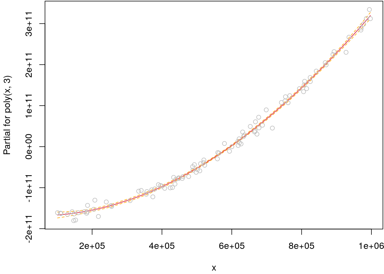

Note that function termplot() plots the so called centered effect of the covariate. The reason is that the orthogonal transformation will center the basis functions around zero, i.e., the linear combination of regression coefficients and the basis functions will also be centered around zero. Moreover, the residuals shown are so called partial residuals, a concept that will be explained later in this script.

The basis functions can be visualized with:

X <- poly(x, 3)
i <- order(x)
par(mar = c(4.1, 4.1, 0.1, 0.1))
matplot(x[i], X[i, ], type = "l", lty = 1,
  xlab = "x", ylab = "B(x)", col = 1:3, lwd = 2)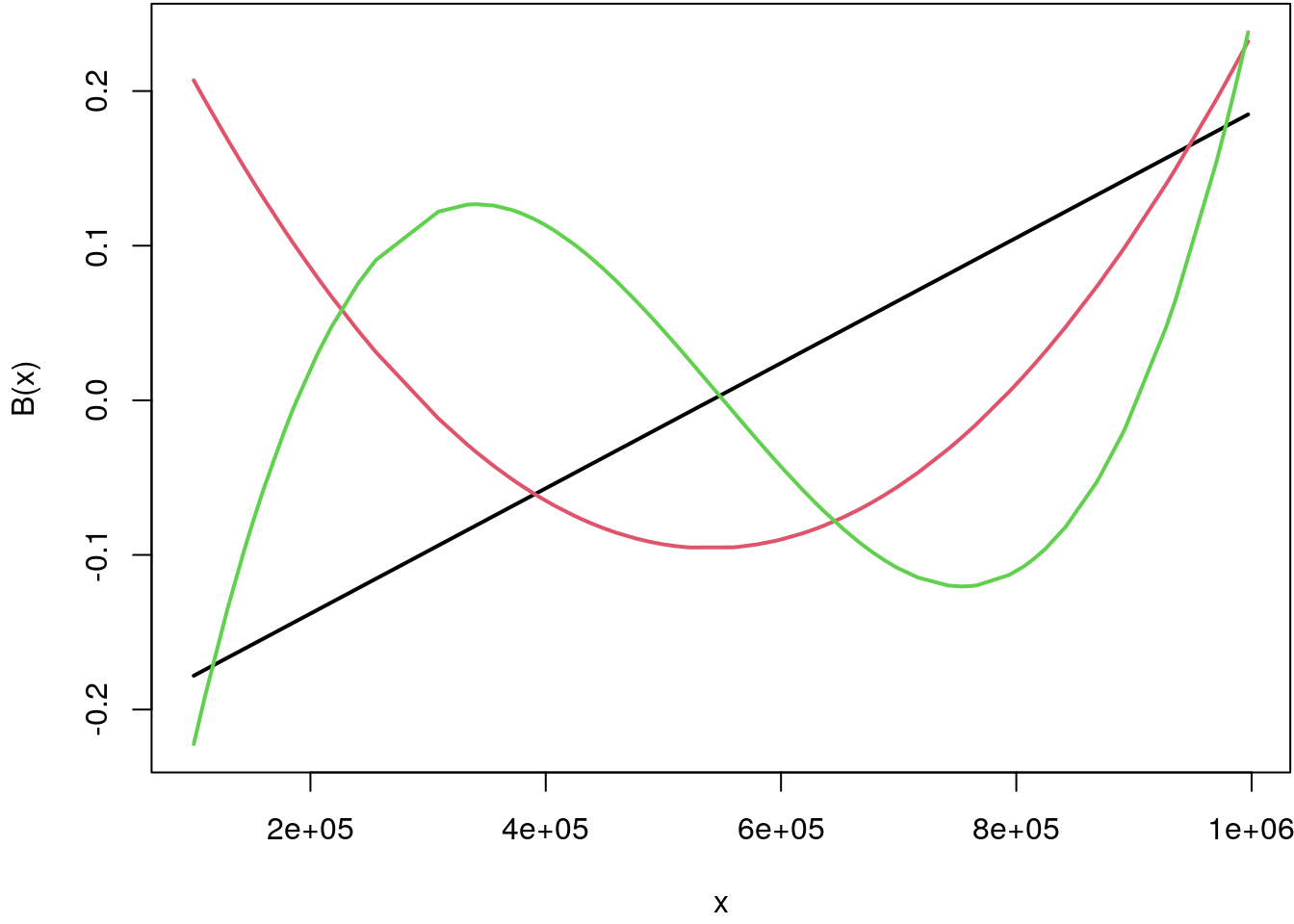

The first basis function is \(x^1\) denoted in black, the second is \(x^2\) denoted in red, and the third is representing \(x^3\) in green. Each of the orthogonal bases is centered around the zero horizontal line. The range on the y-axis that is covered by the three basis functions is only between \(-.2\) and \(.2\), hence, estimation will not lead to numerical instabilities as shown above.

But how should we choose the maximum degree of the polynomial? Pure graphical inspections can be misleading and out-of-sample performance can be poor. A first solution is to use a measure of goodness-of-fit, which also penalizes for model complexity. Readers might already be familiar with the adjusted R-squared, which we already use in the exercise above. For the moment let’s stick to this information criteria, in the upcoming we will introduce more alternatives that are known to have great performance in model and variable selection situations.

Exercise 1.4 Load the MunichRent data and estimate polynomial regression models \[ \texttt{rentsqm}_i = \beta_0 + \sum_{l=1}^{20}\texttt{area}_i^l + \varepsilon_i. \] Again, use the adjusted R-squared to find the best fitting polynomial. Interpret the result.

The data is loaded with

load("data/MunichRent.rda")

Now, we estimate a number of different polynomial models with

L <- 20
rsq <- rep(0, L)
for(l in 1:L) {
  b <- lm(rentsqm ~ poly(area, l), data = MunichRent)
  rsq[l] <- summary(b)$adj.r.squared
}

## Extract best fitting polynomial.
(l <- which.max(rsq))

## [1] 12

b <- lm(rentsqm ~ poly(area, l), data = MunichRent)

## Visualize.
par(mar = c(4.1, 4.1, 0.1, 0.1))
termplot(b, partial.resid = TRUE, se = TRUE, cex = 0.1)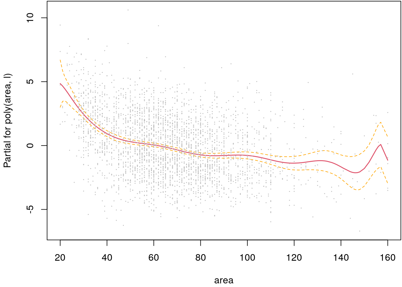

The estimated effect of covariate area seems to be quite appropriate. For small apartments the decrease of net rents per square meter is higher than for large apartments, which is plausible. Only for very large apartments the estimate seems to be a bit unstable, which is caused by the known boundary effects in polynomial regression.

Additive models

Following the last exercise, it is straightforward to include additional covariates with a linear effect into the model \[ \texttt{rentsqm}_i = \beta_0 + f_1(\texttt{area}_i) + \beta_2 \cdot \texttt{yearc}_i + \varepsilon_i. \] Alternatively, we can also estimate the effect of the year of construction nonlinearly. A model using a polynomial of degree 3 is given by \[ \texttt{rentsqm}_i = \beta_0 + \beta_1 \cdot 1/\texttt{area}_i + \beta_2 \cdot \texttt{yearc}_i + \beta_3 \cdot \texttt{yearc}^2_i + \beta_4 \cdot \texttt{yearc}^3_i + \varepsilon_i. \]

Combining the effects of the living area and the year of construction in the functions \[ f_1(\texttt{area}) = \beta_1 \cdot 1 / \texttt{area} \] and \[ f_2(\texttt{yearc}) = \beta_2 \cdot \texttt{yearc} + \beta_3 \cdot \texttt{yearc}^2 + \beta_4 \cdot \texttt{yearc}^3 \] we obtain the model \[ \texttt{rentsqm}_i = \beta_0 + f_1(\texttt{area}_i) + f_2(\texttt{yearc}_i) + \varepsilon_i. \] This a special case of an additive model and in the following we will focus on methods that are almost assumption free for the choice of smooth functions \(f_j( \cdot )\).

Note that the functions \(f_j( \cdot )\) have an identifiability problem. If we add any constant \(a\) to \(\hat{f}_2\) and subtract the same constant from \(\hat{\beta}_0\), the estimated rent per square meter \(\widehat{\texttt{rentsqm}}\) remains unchanged. This implies that the level of the nonlinear function can be arbitrarily changed, e.g., by transforming the explanatory variable. Therefore, it is often useful to require that all functions “are centered around zero”. This condition is automatically fulfilled if all covariates are centered around zero, e.g., by using function scale(). However, as already mention in section Polynomial regression, when function poly() is used to set up the polynomials, each column of the resulting design matrix is centered right away and we do not need to take extra care here.

Exercise 1.5 Load the MunichRent data and estimate additive models of the form \[ \texttt{rentsqm}_i = \beta_0 + f_1(\texttt{area}_i) + f_2(\texttt{yearc}_i) + \varepsilon_i, \] where functions \(f_j( \cdot )\) can be either based on a simple transformation function like log() or sqrt(), or is a polynomial model up to degree \(l = 1, \ldots, 20\). Again, use the adjusted R-squared to find the best fitting polynomial. Interpret the results.

The data is loaded with

load("data/MunichRent.rda")

Now, set up a list of transformer functions and a grid which we can use to find the best model.

trans_fun <- list("exp" = exp, "log" = log, "sqrt" = sqrt,
  "inverse" = function(x) { 1 / x }, "quadratic" = function(x) x^2)

For the polynomial models, we need to extent the list a bit.

for(l in 1:20) {
  poly_fun <- paste0("function(x) { poly(x,", l, ") }")
  trans_fun[[paste0("poly", l)]] <- eval(parse(text = poly_fun))
}

The trick here is to create a character string of the function with the correct degree of the polynomial and save it in object poly_fun. This string is then evaluated with eval(parse()) and the so created function is save in the list. Now it is time to set up the search grid with all combinations.

combos <- expand.grid(
  "area" = names(trans_fun),
  "yearc" = names(trans_fun),
  stringsAsFactors = FALSE
)
print(head(combos))

##        area yearc
## 1       exp   exp
## 2       log   exp
## 3      sqrt   exp
## 4   inverse   exp
## 5 quadratic   exp
## 6     poly1   exp

print(dim(combos))

## [1] 625   2

So in total, we need to estimate 625 linear models and compare them using the adjusted R-squared. In order to avoid numeric problems, e.g., when using the exp() transformation in combination with variable yearc, we scale both covariates such that the maximum value is one in advance.

MunichRent$area_s <- MunichRent$area / max(MunichRent$area)
MunichRent$yearc_s <- MunichRent$yearc / max(MunichRent$yearc)

Now, we write a simple for loop and carry out the grid search.

rsq <- rep(0, nrow(combos))
for(i in 1:nrow(combos)) {
  f <- rentsqm ~ trans_fun[[combos$area[i]]](area_s) + trans_fun[[combos$yearc[i]]](yearc_s)
  b <- lm(f, data = MunichRent)
  rsq[i] <- summary(b)$adj.r.squared
}

## Extract the best fitting model.
i <- which.max(rsq)
print(combos[i, ])

##       area  yearc
## 499 poly19 poly15

## Re-estimate and plot.
f <- rentsqm ~ trans_fun[[combos$area[i]]](area_s) + trans_fun[[combos$yearc[i]]](yearc_s)
b <- lm(f, data = MunichRent)

par(mfrow = c(1, 2), mar = c(4.1, 4.1, 0.1, 0.5))
termplot(b, partial.resid = TRUE, se = TRUE, cex = 0.1)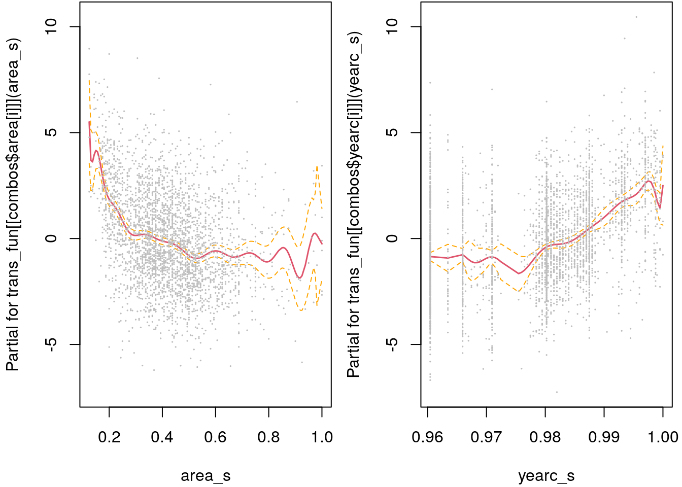

So the adjusted R-squared tends to select models with a very high degree of the polynomial. As already mentioned, this can be quite critical at the borders of the covariates domain, e.g., for very small and very large apartments we see some wiggliness in the functional estimate that is hard to believe. In the upcoming, we will explore tools for model and variable selection that lead to more stable results.

Partial residuals

Partial residuals are an extremely useful tool for exploring whether the influence of \(x_j\) is modeled correctly. The residuals can be visualized by setting argument partial.resid = TRUE in the termplot() function.

The partial residuals regarding covariate \(x_j\) are defined by \[ \hat{\varepsilon}_{x_j,i} = y_i - \hat{\beta}_0 - \hat{\beta}_{j - 1}x_{i, j - 1} - \hat{\beta}_{j + 1}x_{i, j + 1} - \ldots - \hat{\beta}_{k}x_{xik} = \hat{\varepsilon}_i + \hat{\beta}_jx_{ij}. \] In the partial residuals \(\hat{\varepsilon}_{x_j,i}\), all covariate effects with exception of the one associated with \(x_j\) are removed.

Partial residuals for term in our additive model can be calculated with \[\begin{eqnarray*} \hat{\varepsilon}_{\texttt{area}, i} &=& \texttt{rentsqm}_i - \hat{\beta}_0 - \hat{f}(\texttt{yearc}_i) \\ &=& \hat{\varepsilon}_i + \hat{f}(\texttt{area}_i). \end{eqnarray*}\]

Note that users should always inspect the partial residuals to judge if the model fits to the data.

Categorical covariates

For modeling the effect of a covariate \(x \in \{1, \dots, c\}\) with \(c\) categories using dummy coding, we define the \(c-1\) dummy variables \[ x_{i1} = \left\{ \begin{array}{lll} 1 & \mbox{ } & x_i = 1 \\ 0 & \mbox{ } & \mbox{otherwise} \\ \end{array} \right. \quad \dots \quad x_{i,c-1} = \left\{ \begin{array}{lll} 1 & \mbox{ } & x_i = c-1 \\ 0 & \mbox{ } & \mbox{otherwise} \\ \end{array} \right. \] for \(i = 1, \dots, n,\) and include them as explanatory variables in the regression model \[ y_i = \beta_0 + \beta_1 x_{i1} + \ldots + \beta_{i,c-1} x_{i,c-1} + \ldots + \varepsilon_i. \] For reasons of identifiability, we must omit one of the dummy variables, in this case the dummy variable for category \(c\). This category is called reference category. The estimated effects can be interpreted by direct comparison with the (omitted) reference category.

Exercise 1.6 Load the MunichRent data and estimate an additive model of the form \[\begin{eqnarray*} \texttt{rentsqm}_i &=& \beta_0 + f_1(\texttt{area}_i) + f_2(\texttt{yearc}_i) + \\ && \qquad \texttt{locationgood}_i \beta_1 + \texttt{locationtop}_i \beta_2 + \varepsilon_i, \end{eqnarray*}\] where functions \(f_j( \cdot )\) are based on orthogonal polynomials of degree 5. In a second model change the reference category to locationtop. Interpret the results.

The data is loaded with

load("data/MunichRent.rda")

The linear model is estimated with

b <- lm(rentsqm ~ poly(area, 5) + poly(yearc, 5) + location, data = MunichRent)

Note that the reference category is always the first level of the factor variable:

levels(MunichRent$location)

## [1] "normal" "good"   "top"

The model summary output gives

summary(b)

## 
## Call:
## lm(formula = rentsqm ~ poly(area, 5) + poly(yearc, 5) + location, 
##     data = MunichRent)
## 
## Residuals:
##     Min      1Q  Median      3Q     Max 
## -7.1849 -1.3165 -0.1056  1.3336  7.7983 
## 
## Coefficients:
##                  Estimate Std. Error t value Pr(>|t|)    
## (Intercept)       6.82495    0.04775 142.935  < 2e-16 ***
## poly(area, 5)1  -41.86085    2.09638 -19.968  < 2e-16 ***
## poly(area, 5)2   24.01898    2.02020  11.889  < 2e-16 ***
## poly(area, 5)3   -9.93701    2.01138  -4.940 8.21e-07 ***
## poly(area, 5)4    7.50518    2.01639   3.722 0.000201 ***
## poly(area, 5)5   -5.08034    2.00582  -2.533 0.011365 *  
## poly(yearc, 5)1  47.57179    2.09800  22.675  < 2e-16 ***
## poly(yearc, 5)2  26.12098    2.04286  12.786  < 2e-16 ***
## poly(yearc, 5)3  -1.56870    2.01191  -0.780 0.435625    
## poly(yearc, 5)4  -7.48002    2.00817  -3.725 0.000199 ***
## poly(yearc, 5)5  -2.84510    2.01413  -1.413 0.157885    
## locationgood      0.63211    0.07630   8.284  < 2e-16 ***
## locationtop       1.50701    0.23338   6.457 1.23e-10 ***
## ---
## Signif. codes:  0 '***' 0.001 '**' 0.01 '*' 0.05 '.' 0.1 ' ' 1
## 
## Residual standard error: 2.001 on 3069 degrees of freedom
## Multiple R-squared:  0.3281, Adjusted R-squared:  0.3255 
## F-statistic: 124.9 on 12 and 3069 DF,  p-value: < 2.2e-16

So compared to apartments in normal locations apartments in good locations are on average 0.63 more expensive and in top locations 1.51.

We can change the reference category with the relevel() function

MunichRent$location <- relevel(MunichRent$location, ref = "top")

Re-estimate the model and look at the summary output.

b <- lm(rentsqm ~ poly(area, 5) + poly(yearc, 5) + location, data = MunichRent)
summary(b)

## 
## Call:
## lm(formula = rentsqm ~ poly(area, 5) + poly(yearc, 5) + location, 
##     data = MunichRent)
## 
## Residuals:
##     Min      1Q  Median      3Q     Max 
## -7.1849 -1.3165 -0.1056  1.3336  7.7983 
## 
## Coefficients:
##                 Estimate Std. Error t value Pr(>|t|)    
## (Intercept)       8.3320     0.2282  36.519  < 2e-16 ***
## poly(area, 5)1  -41.8608     2.0964 -19.968  < 2e-16 ***
## poly(area, 5)2   24.0190     2.0202  11.889  < 2e-16 ***
## poly(area, 5)3   -9.9370     2.0114  -4.940 8.21e-07 ***
## poly(area, 5)4    7.5052     2.0164   3.722 0.000201 ***
## poly(area, 5)5   -5.0803     2.0058  -2.533 0.011365 *  
## poly(yearc, 5)1  47.5718     2.0980  22.675  < 2e-16 ***
## poly(yearc, 5)2  26.1210     2.0429  12.786  < 2e-16 ***
## poly(yearc, 5)3  -1.5687     2.0119  -0.780 0.435625    
## poly(yearc, 5)4  -7.4800     2.0082  -3.725 0.000199 ***
## poly(yearc, 5)5  -2.8451     2.0141  -1.413 0.157885    
## locationnormal   -1.5070     0.2334  -6.457 1.23e-10 ***
## locationgood     -0.8749     0.2353  -3.718 0.000204 ***
## ---
## Signif. codes:  0 '***' 0.001 '**' 0.01 '*' 0.05 '.' 0.1 ' ' 1
## 
## Residual standard error: 2.001 on 3069 degrees of freedom
## Multiple R-squared:  0.3281, Adjusted R-squared:  0.3255 
## F-statistic: 124.9 on 12 and 3069 DF,  p-value: < 2.2e-16

Now, the interpretation is in terms of the top location. On average, apartments in normal location are -1.51 cheaper compared to apartments in top locations, and apartments in good location are -0.87 cheaper.

We can also plot the estimated effects using the termplot() function.

par(mfrow = c(1, 3), mar = c(4.1, 4.1, 0.1, 0.5))
termplot(b, partial.resid = TRUE, se = TRUE, cex = 0.1)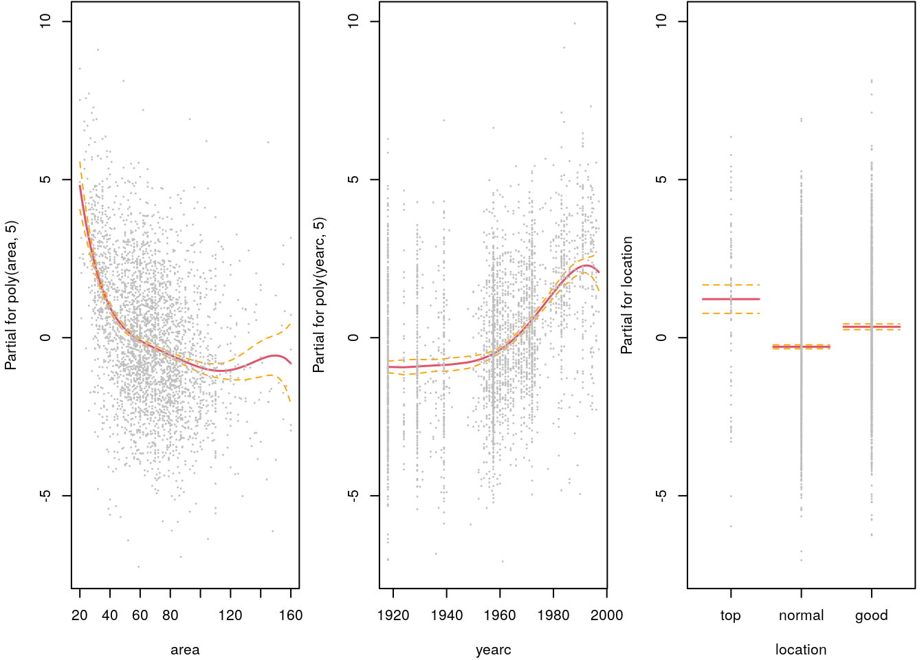

The effect plot of the categorical variable location nicely depicts the difference between normal, good and top locations.

Interactions

An interaction between covariates exists if the effect of a covariate depends on the value of at least one other covariate. Consider \[ y = \beta_0 + \beta_1x + \beta_2z + \beta_3xz + \varepsilon \] The term \(\beta_3xz\) is called an interaction between \(x\) and \(z\). The terms \(\beta_1x\) and \(\beta_2z\) depend on only one variable and are called main effects.

Impact of an interaction term when, e.g., \(x\) changes by an amount \(d\) \[ \begin{array}{lll} E(y | x + d,z) - E(y | x, z) & = & \beta_0 +\beta_1 (x + d) + \beta_2z + \beta_3(x + d)z \\ && - \beta_0 -\beta_1x - \beta_2z - \beta_3xz \\ & = & \beta_1d + \beta_3dz. \\ \end{array} \] Now we can distinguish between the two cases \(\beta_3=0\) and \(\beta_3 \neq 0\):

In the case \(\beta_3=0\), the interaction is dropped from the model and the expected change \(\beta_1 d\) is independent from the specific value of the second covariate \(z\).
In the case \(\beta_3 \neq 0\), the expected change \(\beta_1 d + \beta_3 d z\) does not only depend on the amount \(d\), but also on the value of the covariate z.

Therefore, an interaction is always needed if the effect of the change of a variable is also dependent on the value of another variable.

A general interaction model can be written as \[ y = \beta_0 + \beta_1z_1 + \beta_2z_2 + f_1(x) + f_2(x)z_1 + f_3(x)z_2 + \ldots + \varepsilon, \] where \(f_1\), \(f_2\), and \(f_3\) are again linear or nonlinear functions and covariate \(z\) is a three level categorical covariate. The model consists of the following effects:

\(f_1(x)\): Effect of the continuous variable \(x\), if \(z = 3\) (reference category).
\(\beta_1 + f_1(x)+f_2(x)\): Effect of the continuous variable \(x\), if \(z = 1\).
\(\beta_2 + f_1(x)+f_3(x)\): Effect of the continuous variable \(x\), if \(z = 2\).
\(\beta_1 + f_2(x)\): Varying effect of the level \(z = 1\) depending on \(x\). The effect has to be interpreted as a difference relative to the reference category \(z = 3\).
\(\beta_2 + f_3(x)\): Varying effect of the level \(z=2\), depending on \(x\).

Exercise 1.7 Load the MunichRent data and estimate an additive interaction model with \[\begin{eqnarray*} \texttt{rentsqm}_i &=& \beta_0 + \texttt{locationgood}_i \beta_1 + \texttt{locationtop}_i \beta_2 +\\ && \quad f_1(\texttt{area}_i) + f_2(\texttt{area}_i)\texttt{locationgood}_i + f_3(\texttt{area}_i)\texttt{locationtop}_i + \varepsilon_i, \end{eqnarray*}\] where functions \(f_j( \cdot )\) are based on orthogonal polynomials of degree 3. Visualize and interpret the results.

The data is loaded with

load("data/MunichRent.rda")

The linear model is estimated with

b <- lm(rentsqm ~ poly(area, 3)*location, data = MunichRent)

To visualize the effects of location and the area of the apartment, we need to predict for each level of the categorical covariate.

## Create a new data frame for prediction.
nd <- MunichRent[, c("area", "location", "rentsqm")]

## Predict for each level of location including
## 95% confidence intervals.
nd$location <- "normal"
nd$pnormal <- predict(b, newdata = nd, interval = "confidence")

nd$location <- "good"
nd$pgood <- predict(b, newdata = nd, interval = "confidence")

nd$location <- "top"
nd$ptop <- predict(b, newdata = nd, interval = "confidence")

## Plot the effects
par(mar = c(4.1, 4.1, 0.1, 0.1))
i <- order(nd$area)
nd <- nd[i, ]
plot(rentsqm ~ area, data = nd, col = rgb(0.1, 0.1, 0.1, alpha = 0.1), cex = 0.5)
matplot(nd$area, nd$pnormal, type = "l", lty = c(1, 2, 2), col = 1,
  lwd = c(2, 1, 1), add = TRUE)
matplot(nd$area, nd$pgood, type = "l", lty = c(1, 2, 2), col = 2,
  lwd = c(2, 1, 1), add = TRUE)
matplot(nd$area, nd$ptop, type = "l", lty = c(1, 2, 2), col = 3,
  lwd = c(2, 1, 1), add = TRUE)
legend("topright", c("normal", "good", "top"),
  lwd = 2, col = 1:3, bty = "n")
rug(nd$area)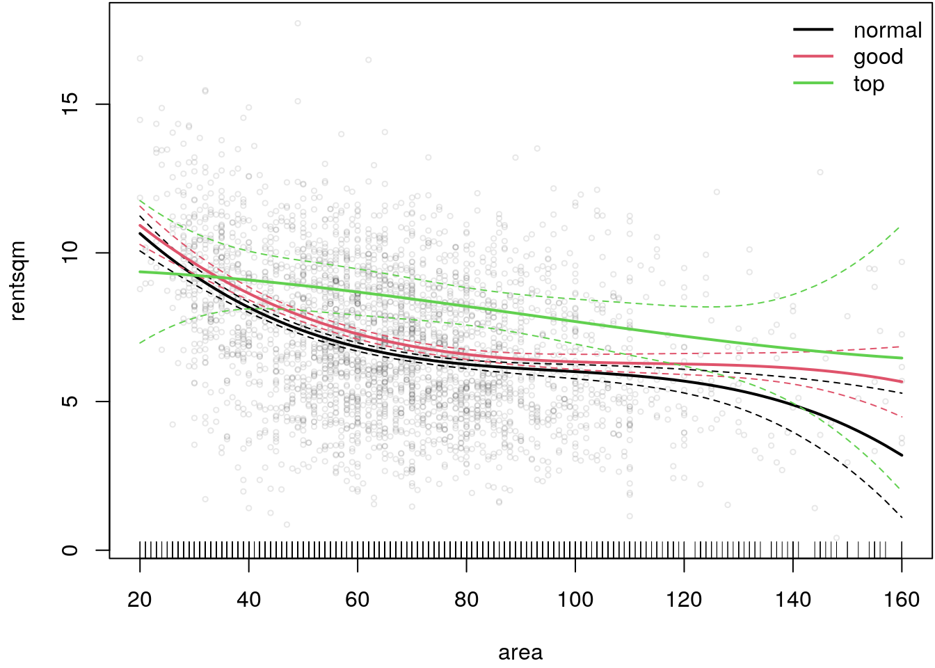

The plot indicates that there is a varying effect of area and location on the net rent per square meter. The greatest difference is between top apartments and apartments in normal or good location. It seems like the effect of area for apartments in top location is much flatter and average rents are clearly higher. The rug plot at the bottom additionally shows the distribution of covariate area, indicating that for very large apartments uncertainty about the net rent is the highest, as shown by the 95% confidence intervals.

1.6 Diagnostic plots

Any patterns in the residuals reflect extra structure that is not accommodated by the model.

A simple diagnostic check is to plot the fitted values against the response observations. The residuals should follow the zero horizontal line and should be evenly scattered.
A trend in the mean would violate the assumption of independent response variables, usually results from an erroneous model structure.
A trend in the variability of the residuals suggests that the variance of the response is related to its mean, violating the constant variance assumption.
Transformation of the response or a GLM may help.
Another option to check the distributional assumption is to use so called quantile-quantile plots. The cumulative distribution function of a random variable \(X\) is \[ F(x) = P(X \leq x) = p. \] The inverse \(Q\) is called the quantile function. If \(F\) is a one to one function the inverse \(Q\) is uniquely determined \[ Q(p) = x \,\, \text{if} \,\, F(x) = p. \] The idea is to plot the theoretical quantiles against the quantiles we generated from the residuals. If the residuals are normally distributed then the resulting plot should look like a straight line relationship.
Residuals are not always adequate to confirm model assumptions. In most cases, the correlation is negligible, but this is not the case with the heteroscedasticity. Verification of homoscedastic errors is problematic, as heteroscedastic residuals are in general not an indicator for heteroscedastic errors. An obvious solution of the heteroscedasticity problem is standardization. The vector of residuals is \[ \boldsymbol{\varepsilon} = \mathbf{y} - \hat{\mathbf{y}} = \mathbf{y} - \mathbf{H}\mathbf{y} = (\mathbf{I} - \mathbf{H})\mathbf{y}, \] where \[ Cov(\boldsymbol{\varepsilon}) = Cov((\mathbf{I} - \mathbf{H})\mathbf{y}) = (\mathbf{I} - \mathbf{H}) \sigma^2 (\mathbf{I} - \mathbf{H})^\top =\sigma^2 (\mathbf{I} - \mathbf{H}). \] \(\widehat{\text{st.dev.}}(\varepsilon_i) = \hat{\sigma} \sqrt{1 - H_{ii}}.\) The \(i\)th internally studentized (normalized) residual is \[ \varepsilon_i^{\star} \equiv \frac{\varepsilon_i}{\widehat{\text{st.dev.}}(\varepsilon_i)} = \frac{\varepsilon_i}{\hat{\sigma} \sqrt{1 - H_{ii}}}. \] Under normality and homoscedasticity \(\varepsilon_i^{\star}\) should behave like a \(N(0, 1)\) sample if the model is correct.

Using the lm() function we have all the diagnostic plots (and more) directly in place. For example, residual diagnostics of the Munich rent data model can be visualized with

load("data/MunichRent.rda")

## Model with two nonlinear effects.
b <- lm(rentsqm ~ poly(area, 3) + poly(yearc, 3), data = MunichRent)

## Diagnostic plots, see also ?plot.lm.
par(mfrow = c(2, 2))
plot(b)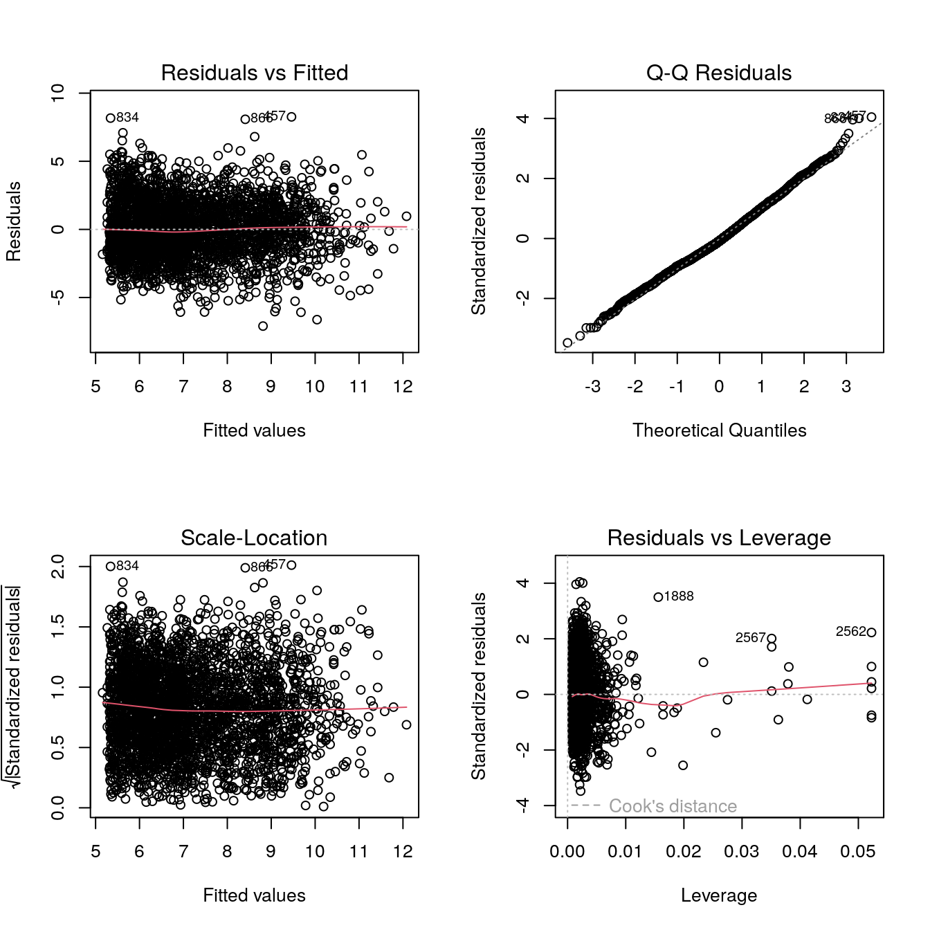

The diagnostic plots indicate, that the model fits quite well to the data. The plots of fitted values vs. residuals suggest that there is no pronounced visible trend. The Q-Q plot indicates that the distributional assumptions of the linear model are largely fulfilled. However, the fitted values vs. residual plots also indicate that there might be a heteroskedasticity problem, i.e., compared to small fitted values the residuals fluctuate around the zero horizontal line much less. Models that can account for this will be discussed in upcoming chapters.

1.7 Heteroskedasticity

In many applications it can happen that the uncertainty, i.e. the variance of the error term, is dependent on covariates. In this case we speak of a heteroscedasticity problem. Fortunately, with the help of weighted OLS we can still estimate valid models and the inference of the regression parameters remains valid.

Weighted least squares

This method is comparatively simple, but before we derive the exact estimation algorithm we take a closer look at the heteroscedasticity problem on simulated data.

## Set the seed.
set.seed(456)

## Number of observations.
n <- 200

## Simulate simple regression model
## with heteroskedastic error term.
x <- runif(n, -1, 1)
y <- 1.2 + 0.1 * x + rnorm(n, sd = exp(-1 + 2 * x))

## Visualize.
par(mar = c(4.1, 4.1, 0.1, 0.1))
plot(x, y)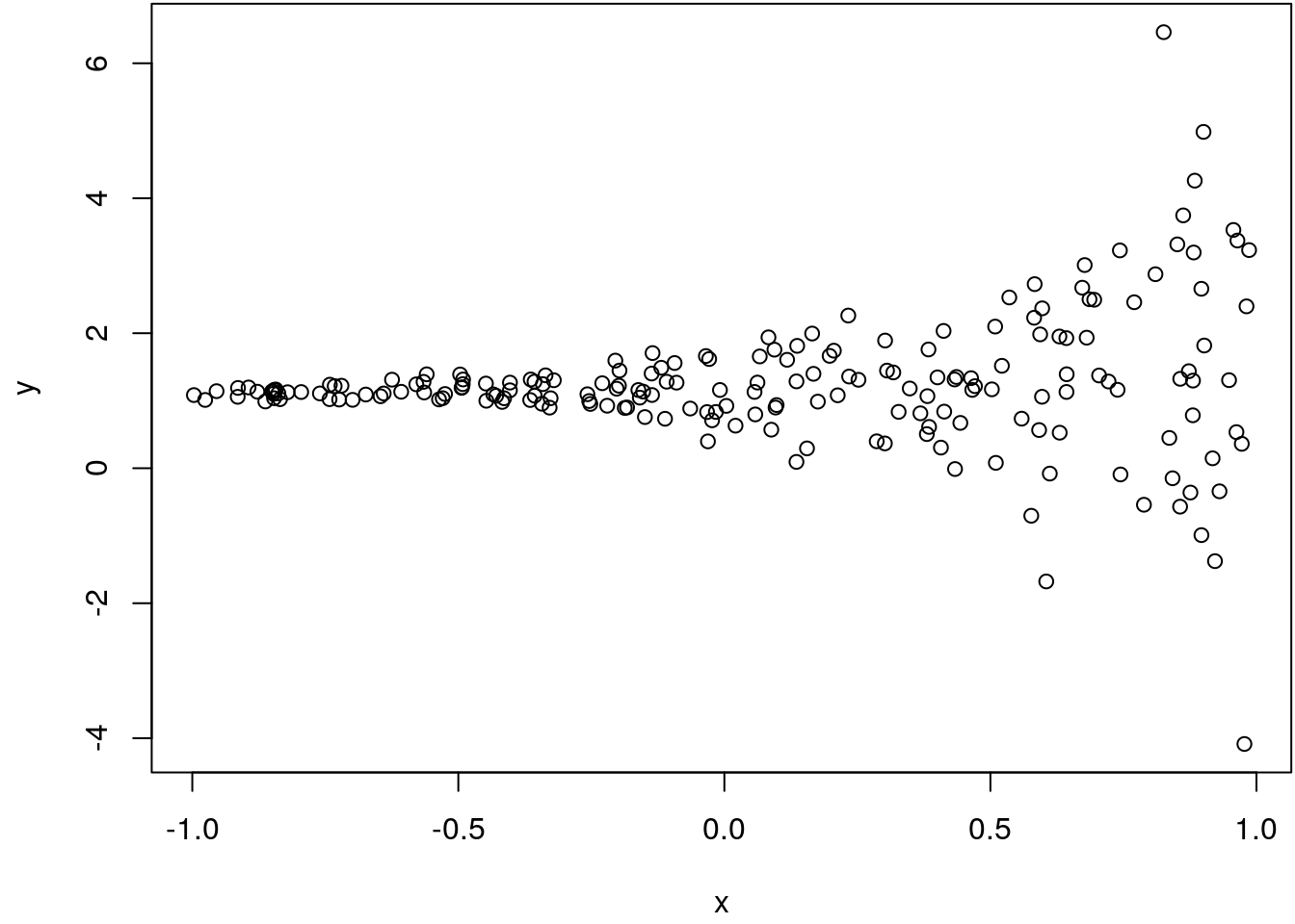

The scatterplot clearly shows that with increasing values of x the uncertainty, the scattering, of the response y increases. In this visualization it is also quite apperent, that a linear regression model will probably underestimate the significance of the slope coefficient for covariate x, because the mean regression is pretty sensible to large positive and negative observations, as is the case here.

Actually there a couple of ways how to account for heteroskedasticity, but let’s start with this particular weighted least squares method. Instead of assuming a constant variance parameter \(\sigma^2\) we relax the model to \[ y_i = \beta_0 + \beta_1x_{i1} + \ldots + \beta_kx_{ik} + \varepsilon_i \] and \[ \varepsilon_i^2 = \sigma^2 \exp(\gamma_0 + \gamma_1x_{i1} + \ldots + \gamma_kx_{ik}) \tilde{\varepsilon}_i, \] i.e., the variance is a function of the covariates. Here, the error term \(\tilde{\varepsilon}_i\) is assumed to have mean equal to unity. Further, if we assume independence of the covariates \(\mathbf{x}_i\) and \(\tilde{\varepsilon}_i\) we can set up a model for the variance with \[ \log(\varepsilon^2_i) = \gamma_0 + \gamma_1x_{i1} + \ldots + \gamma_kx_{ik} + \tilde{\varepsilon}_i. \] If we can compute estimates \(\hat{\gamma}_j, j = 1, \ldots, k\), we can adjust the original model with weights \(\hat{w}_i^{-1}\) and \[ \hat{w}_i = \exp(\hat{\gamma}_0 + \hat{\gamma}_1x_{i1} + \ldots + \hat{\gamma}_kx_{ik}). \] Why does this work? The reason is that in the case of heteroskedasticity the conditional variance equals to \[ Var(\varepsilon_i | \mathbf{x}_i) = E(\varepsilon_i^2 | \mathbf{x}_i) = \sigma^2\exp(\gamma_0 + \gamma_1x_{i1} + \ldots + \gamma_kx_{ik}) = \sigma^2w_i. \] Therefore, the variance of \(\varepsilon_i / \sqrt{w_i}\) is \(\sigma^2\) since \[ E((\varepsilon / \sqrt{w_i})^2) = E(\varepsilon_i^2)/w_i = (\sigma^2w_i) / w_i = \sigma^2. \] This means if we have an estimate \(\hat{w}_i\) we can specify the weighted model with \[ y/\sqrt{\hat{w}_i} = \beta_0/\sqrt{\hat{w}_i} + \beta_1x_{i1}/\sqrt{\hat{w}_i} + \ldots + \beta_kx_{ik}/\sqrt{\hat{w}_i} + \varepsilon_i/\sqrt{\hat{w}_i} \] and obtain a heteroskedastic corrected model with valid inference, i.e., the estimators of the weighted version of the model is more efficient. This is also called the feasible generalized least squares (GLS) estimator. Intuitively, we simply weigh observations with high variance less.

The weighted least squares algorithm can be summarized by the following:

Estimate the original model using lm().
Extract the residuals with residuals() and compute \(\log(\hat{\varepsilon}^2)\).
Estimate the variance model to obtain \(\hat{\gamma}_j\), extract the fitted values using fitted().
Take the exp() of the fitted values of the variance model to obtain \(\hat{w}_i\).
Multiply the response \(\mathbf{y}\) and the design matrix \(\mathbf{X}\) with \(1/\sqrt{\hat{w}_i}\). Or instead if the fitting routine multiplies the residual sum of squares with weights \[ \sum_{i = 1}^n(y_i - \beta_0 - \beta_1x_{i1} - \ldots - \beta_kx_{ik}) / \hat{w}_i \] it is easy to see that this is equivalent as pre-multiplying the data with \(1/\sqrt{\hat{w}_i}\) by bringing \(1/\hat{w}_i\) inside the squared residuals.
Iterate steps 1.-5. until convergence.

It is now time to implement this algorithm using a simple while() loop:

## Heteroskedastic linear model fitting function.
## Argument eps controls stopping of the while loop.
hetlm <- function(formula, data = NULL, eps = 1e-05, ...) {
  ## Step 1, initial linear model.
  b <- lm(formula, data = data, ...)

  ## Extract fitted values to measure change of fit
  ## at the end of the while loop.
  fit0 <- fitted(b)

  ## The variance model formula,
  ## note e2 will be set up within the while loop.
  formula_sigma2 <- update(formula, log_e2 ~ .)

  ## Start the while loop, therefore initialize
  ## change parameter.
  change <- 1

  ## Save number of iterations.
  iter <- 0
  while(eps < change) {
    ## Extract log-squared residuals.
    ## Note that the doubled arrow "<<-" assigns variables
    ## to the global environment. This way object log_e2,
    ## and h below is available for fitting the model
    ## with lm().
    log_e2 <<- log(residuals(b)^2)

    ## Estimate variance model.
    m <- lm(formula_sigma2, data = data, ...)

    ## Compute the weights.
    h <<- exp(fitted(m))

    ## Estimate weighted linear model.
    b <- lm(formula, weights = 1/h, data = data, ...)

    ## Extract fitted values and compute
    ## relative change value.
    fit1 <- fitted(b)
    change <- mean(abs((fit1 - fit0) / fit0))

    ## Overwrite initial fitted values.
    fit0 <- fit1

    iter <- iter + 1
  }

  ## Delete log_e2 and h from global environment.
  rm(list = c("log_e2", "h"), envir = .GlobalEnv)

  ## Even a bit more technical, change the call of the "lm"
  ## object, so we can use the predict() method.
  cl <- match.call()
  b$call$data <- m$call$data <- cl$data

  ## Return models for the mean and the variance.
  rval <- list("mean" = b, "variance" = m, "iterations" = iter)
  return(rval)
}

Let’s test the new function on our simulated data.

## Model without accounting for heteroskedasticity.
b0 <- lm(y ~ x)
summary(b0)

## 
## Call:
## lm(formula = y ~ x)
## 
## Residuals:
##     Min      1Q  Median      3Q     Max 
## -5.5296 -0.2638  0.0174  0.2214  5.0503 
## 
## Coefficients:
##             Estimate Std. Error t value Pr(>|t|)    
## (Intercept)  1.22847    0.07168  17.137   <2e-16 ***
## x            0.22044    0.12379   1.781   0.0765 .  
## ---
## Signif. codes:  0 '***' 0.001 '**' 0.01 '*' 0.05 '.' 0.1 ' ' 1
## 
## Residual standard error: 1.003 on 198 degrees of freedom
## Multiple R-squared:  0.01576,    Adjusted R-squared:  0.01079 
## F-statistic: 3.171 on 1 and 198 DF,  p-value: 0.07649

## Now using the new model fitting routine.
b <- hetlm(y ~ x)
summary(b$mean)

## 
## Call:
## lm(formula = formula, weights = 1/h)
## 
## Weighted Residuals:
##     Min      1Q  Median      3Q     Max 
## -4.9762 -1.3627  0.0219  1.5156  5.9218 
## 
## Coefficients:
##             Estimate Std. Error t value Pr(>|t|)    
## (Intercept)  1.19267    0.03297  36.173   <2e-16 ***
## x            0.09445    0.04411   2.141   0.0335 *  
## ---
## Signif. codes:  0 '***' 0.001 '**' 0.01 '*' 0.05 '.' 0.1 ' ' 1
## 
## Residual standard error: 1.851 on 198 degrees of freedom
## Multiple R-squared:  0.02263,    Adjusted R-squared:  0.0177 
## F-statistic: 4.585 on 1 and 198 DF,  p-value: 0.03347

summary(b$variance)

## 
## Call:
## lm(formula = formula_sigma2)
## 
## Residuals:
##      Min       1Q   Median       3Q      Max 
## -11.1272  -1.0447   0.7396   1.4643   3.5573 
## 
## Coefficients:
##             Estimate Std. Error t value Pr(>|t|)    
## (Intercept)  -3.2465     0.1653  -19.64   <2e-16 ***
## x             3.6123     0.2854   12.66   <2e-16 ***
## ---
## Signif. codes:  0 '***' 0.001 '**' 0.01 '*' 0.05 '.' 0.1 ' ' 1
## 
## Residual standard error: 2.311 on 198 degrees of freedom
## Multiple R-squared:  0.4472, Adjusted R-squared:  0.4445 
## F-statistic: 160.2 on 1 and 198 DF,  p-value: < 2.2e-16

print(b$iterations)

## [1] 4

## Visualize the effects.
par(mfrow = c(1, 2), mar = c(4.1, 4.1, 4.1, 1.1))
termplot(b$mean, se = TRUE, partial.resid = TRUE, main = "mu")
termplot(b$variance, se = TRUE, partial.resid = TRUE, main = "sigma^2")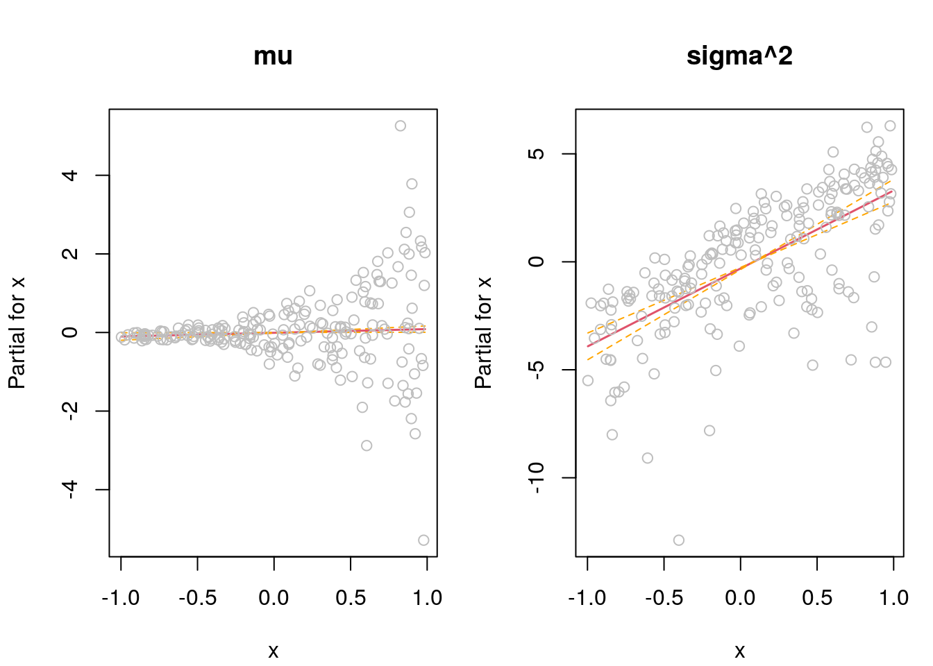

Note that the initial model overestimated the slope coefficient of covariate x and is not really significant. The weighted version of the linear model accounting for the inherent heteroskedasticity could recover the true slope parameter quite well. The effect plots for the mean and the variance model look very reasonable (since we know how the data was generated). The algorithm converged after \(4\) iterations.

Breusch-Pagan test for heteroskedasticity

Sometimes a raw graphical inspection, e.g. using standardized residuals, to detect the heteroskedasticity problem is not possible. In such cases we need a more automated way for detection in form of a test. There are a couple of test in the literature, however, many of them do not account for dependency of the variance on covariates. Here we restrict to one particular test, the Breusch-Pagan test.

This Breusch-Pagan test is based on the variance model \[ \varepsilon_i^2 = \gamma_0 + \gamma_1x_{i1} + \ldots + \gamma_kx_{ik} + \tilde{\varepsilon}_i. \] Note, that we do not take the logarithm of the left side of the equation this time. If there is no heteroskedasticity problem all coefficients \(\gamma_j, j = 1, \ldots, k\) should be zero. Hence, we specify \[ H_0: \gamma_1 = \gamma_2 = \ldots = \gamma_k = 0 \] and test against \[ H_1: \gamma_j \not= 0 \text{ for at least one } j. \] To test the hypothesis, we need to perform the following steps:

Estimate a simple linear model using lm().
Compute the squared residuals \(\hat{\varepsilon}^2\) using residuals().
Estimate the linear model \[ \hat{\varepsilon}_i^2 = \gamma_0 + \gamma_1x_{i1} + \ldots + \gamma_kx_{ik} + \tilde{\varepsilon}_i. \]
The test is computed using the \(R^2\) of the variance model, the test statistic is \[ LM = n \cdot R^2 \sim \chi_{k - 1}^2 \] and is asymptotically \(\chi^2\)-distributed with \(k - 1\) degrees of freedom. The \(R^2\) can be extracted using the summary() method for "lm" objects.

Note that this test is asymptotic in nature, so it is only valid for “large” sample sizes. What “large” means depends on the application. For smaller sample sizes we can also use a simple \(F\)-test for significance of all covariates in the variance model. Although the Breusch-Pagan test is implemented in a couple of R packages we show the implementation from scratch.

bp_test <- function(formula, ...) {
  ## Estimate mean model.
  b <- lm(formula, ...)
  
  ## Extract and square residuals.
  e2 <<- residuals(b)^2

  ## Variance model formula.
  formula_sigma2 <- update(formula, e2 ~ .)

  ## Fit variance model.
  m <- lm(formula_sigma2, ...)

  ## Extract the test statistic.
  LM <- nobs(m) * summary(m)$r.squared

  ## Compute the p-value.
  df_LM <- length(coefficients(m)) - 1
  pval_LM <- 1 - pchisq(LM, df_LM)

  ## And the F-statistic.
  F <- as.numeric(summary(m)$fstatistic)
  pval_F <- pf(F[1L], F[2L], F[3L], lower.tail = FALSE)

  ## Clean up global environment.
  rm(list = "e2", envir = .GlobalEnv)

  rval <- list(
    "LM" = c("LM-statistic" = LM, "df" = df_LM, "p-value" = pval_LM),
    "F" = c("F-statistic" = F[1], "df" = F[3], "p-value" = pval_F)
  )

  return(rval)
}

The test on the simulated data example gives

bp_test(y ~ x)

## $LM
## LM-statistic           df      p-value 
## 2.829721e+01 1.000000e+00 1.040460e-07 
## 
## $F
##  F-statistic           df      p-value 
## 3.263108e+01 1.980000e+02 4.040007e-08

The test clearly identifies heteroskedasticity since the p-values are very small.

Exercise 1.8 Load the ZambiaNutrition data and estimate the following additive model \[ \texttt{stunting}_i = \beta_0 + f_1(\texttt{mbmi}_i) + f_2(\texttt{agechild}_i) + \varepsilon_i, \] where functions \(f_j( \cdot )\) are modeled as orthogonal polynomials of degree \(3\). Test for heteroskedasticity with significance level \(\alpha = 0.05\). If the test is positive, i.e., we need to suspect that there is a heteroskedasticity problem, use the weighted least squares algorithm to estimate a corrected model. Compare the estimated effects of the orginal and the corrected model in this case.

## Load the data.
load("data/ZambiaNutrition.rda")

## Use the Breusch-Pagen test.
bp_test(stunting ~ poly(mbmi, 3) + poly(agechild, 3), data = ZambiaNutrition)

## $LM
## LM-statistic           df      p-value 
##  13.30664083   6.00000000   0.03841682 
## 
## $F
##  F-statistic           df      p-value 
## 2.220667e+00 4.840000e+03 3.835191e-02

The p-values are smaller than the specified significance level \(\alpha = 0.05\), hence, we need to suspect that the variance is not constant and depends on covariates and that the usual standard errors are not reliable. Now, we estimate the corrected model using the hetlm() model fitting function.

b <- hetlm(stunting ~ poly(mbmi, 3) + poly(agechild, 3), data = ZambiaNutrition)

The algorithm cycles through \(7\) iterations. The uncorrected model is estimated by

m <- lm(stunting ~ poly(mbmi, 3) + poly(agechild, 3), data = ZambiaNutrition)

The estimated effects can be directly compared with

par(mfrow = c(2, 2), mar = c(4.1, 4.1, 4.1, 1.1))
termplot(b$mean, term = 1, partial.resid = TRUE, se = TRUE,
  main = "Corrected", pch = ".")
termplot(m, term = 1, partial.resid = TRUE, se = TRUE,
  main = "Uncorrected", pch = ".")
termplot(b$mean, term = 2, partial.resid = TRUE, se = TRUE,
  main = "Corrected", pch = ".")
termplot(m, term = 2, partial.resid = TRUE, se = TRUE,
  main = "Uncorrected", pch = ".")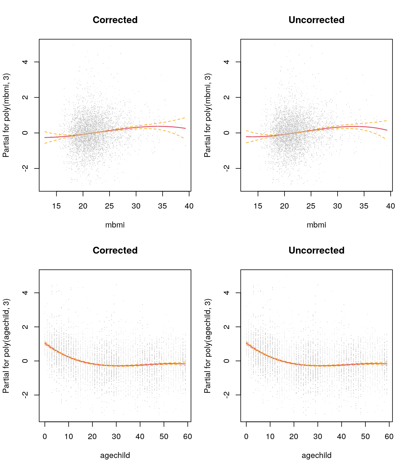

## Show estimated coefficients.
print(round(cbind("corrected" = coef(b$mean), "uncorrected" = coef(m)), 3))

##                    corrected uncorrected
## (Intercept)            0.000       0.000
## poly(mbmi, 3)1         8.460       8.532
## poly(mbmi, 3)2        -0.974      -1.118
## poly(mbmi, 3)3        -1.000      -1.374
## poly(agechild, 3)1   -18.000     -18.063
## poly(agechild, 3)2    15.728      15.695
## poly(agechild, 3)3    -5.736      -5.663

The estimated effects look quite similar for the corrected and the uncorrected model, maybe the effects of the corrected model are slightly smoother. This is also reflected by the estimated coefficients, which only show minor differences.

Considering 95% predictive intervals of covariate agechild when holding mbmi fixed at its mean gives

## Generate new data for predcition.
nd <- ZambiaNutrition
nd$mbmi <- mean(nd$mbmi)
nd <- nd[order(nd$agechild), ]

## Predict uncorrected model.
p_m <- predict(m, newdata = nd, interval = "prediction")

## And the corrected model.
## First, we need to compute the weights from the
## variance model.
h <- exp(predict(b$variance, newdata = nd))

## Now, run predict for the mean model.
p_b <- predict(b$mean, newdata = nd, interval = "prediction", weights = 1/h)

## Add partial residuals to the plot.
e <- residuals(b$mean) + p_b[, "fit"]

## Compare predictions in one plot.
par(mar = c(4.1, 4.1, 0.1, 0.1))
plot(ZambiaNutrition$agechild, e, pch = ".", ylim = range(c(p_m, p_b)),
  xlab = "agechild", ylab = "stunting")
matplot(nd$agechild, p_m, type = "l", lty = c(1, 2, 2), col = 4, add = TRUE)
matplot(nd$agechild, p_b, type = "l", lty = c(1, 2, 2), col = 2, add = TRUE)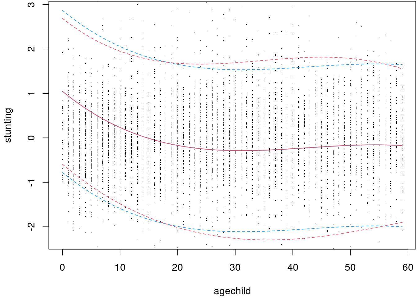

Here, the 95% prediction intervals are clearly different. The prediction interval of the corrected model is wider for agechild ranging form \(20\) to almost \(60\) and smaller below \(20\). Accounting for heteroskedasticiy definitely has an influence on inference in this example.