Chapter 4 Quantile regression
In many situations, regression to the mean is not effective, for example when it comes to explaining income with covariates. First, income clearly follows a skewed distribution which is critical with the assumptions for the errors \(\varepsilon_i\) in the linear model and second, we are not necessarily interested in average income, which can be significantly biased, but rather in median income, or other quantiles. A similar example is the weight of newborn children, here we are more interested in whether a child is still on the lowest percentile or already below it. Quantile regression (Koenker 2005) is the right method in such situations, especially since multimodal distributions can easily be modelled in addition.
In section Heteroskedasticity we have actually already got to know a method to model quantiles. We specified a model accounting for heteroskedastity \[ y_i = \mathbf{x}_i^{\top}\boldsymbol{\beta} + \exp(\mathbf{x}_i^{\top}\boldsymbol{\gamma})\varepsilon_i, \] here \(\varepsilon_i \sim N(0, 1)\) and \(Var(y | \mathbf{x}_i) = \exp(\mathbf{x}_i^{\top}\boldsymbol{\gamma})\). Sure, with the estimate for the variance function we can easily compute any quantile of the normal distribution, e.g., to obtain 95% credible intervals, using \[ \mathbf{x}_i^{\top}\hat{\boldsymbol{\beta}} + z_{\tau}\exp(\mathbf{x}_i^{\top}\hat{\boldsymbol{\gamma}}). \] Here, \(z_{\tau}\) for \(\tau \in (0, 1)\) is the \(\tau\)-quantile of the standard normal distribution. However, considering extreme quantiles this approach is not always a good way to model all characteristics of the distribution.
To illustrate the problem, let’s first have a look at the following scatter-plot of log income versus age as provided in the SemiPar package (Wand 2018).
## Load the data.
data("age.income", package = "SemiPar")

## Create a scatter-plot.
par(mar = c(4.1, 4.1, 0.1, 0.1))
plot(log.income ~ age, data = age.income)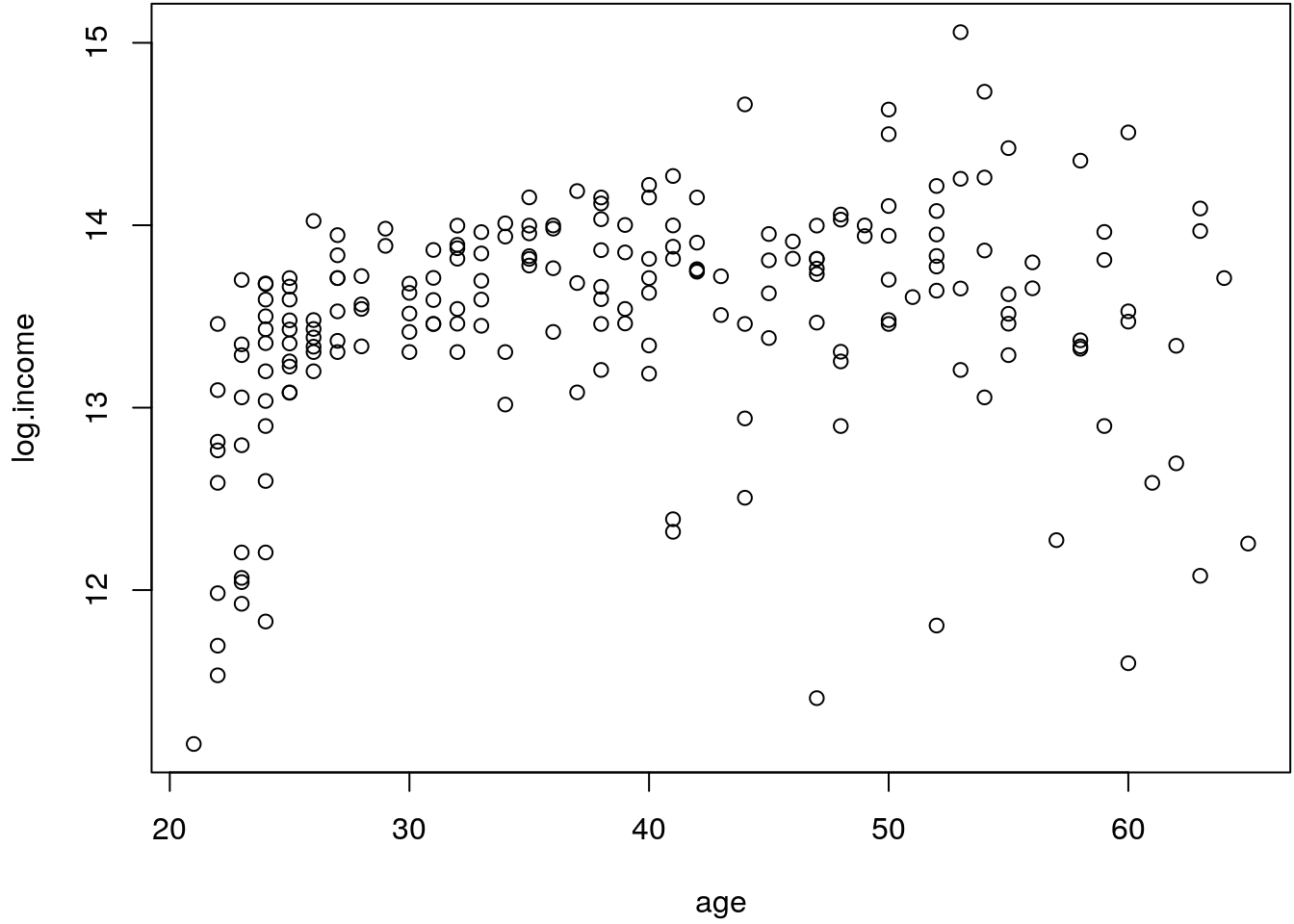
The plot clearly shows that for ages \(<30\) years income increases very quickly. For ages
\(>30\) years it seems like there is not so much variation in the mean income anymore, but
the variance definitely increases, although we are already looking at log income data (the
logarithmic transformation stabilizes the variances in a lot of applications such that
modeling the variance in terms of covariates in not necessary anymore). It seems like,
e.g., for the lower \(10\)% incomes that there is also a decline for people \(>50\)
years. Hence, a constant variance assumption is not fulfilled in this example, we can also
test this using the Breusch-Pagan test for heteroskedasticity assuming a nonlinear
influence of age on log.income.
bp_test(log.income ~ poly(age, 5), data = age.income)## $LM
## LM-statistic df p-value
## 16.8159055 5.0000000 0.0048625
##
## $F
## F-statistic df p-value
## 3.556480e+00 1.990000e+02 4.207276e-03The small p-values suggest, that there is a heteroskedasticity problem. Hence, in order to estimate 95% credible intervals, we need to account for the changing variance, e.g., by using the two-step Weighted least squares algorithm. The following code estimates the linear model and the model for the variance parameter. With the estimated mean and the variance model we can then compute several quantiles of the fitted normal distributions.
## Estimate models.
b <- hetlm(log.income ~ poly(age, 5), data = age.income)

## Extract fitted variance.
sigma2 <- exp(fitted(b$variance))

## Compute several predicted quantiles using qnorm().
tau <- c(0.025, 0.5, 0.975)
q <- list()
for(j in tau) {
  q[[paste0(j * 100, "%")]] <- qnorm(j, mean = fitted(b$mean), sd = sqrt(sigma2))
}

## Create a matrix from the list.
q <- do.call("cbind", q)
print(head(q))
## 2.5% 50% 97.5%
## 1 10.34522 12.18743 14.02965
## 2 11.52143 12.55968 13.59792
## 3 11.52143 12.55968 13.59792
## 4 11.52143 12.55968 13.59792
## 5 11.52143 12.55968 13.59792
## 6 11.52143 12.55968 13.59792## And plot.
par(mar = c(4.1, 4.1, 0.1, 0.1))
plot(log.income ~ age, data = age.income)
matplot(age.income$age, q, type = "l", lty = c(2, 1, 3), col = 1, lwd = 2, add = TRUE)
legend("topleft", paste0(tau*100, "%"), lwd = 2, lty = c(2, 1, 3), bty = "n")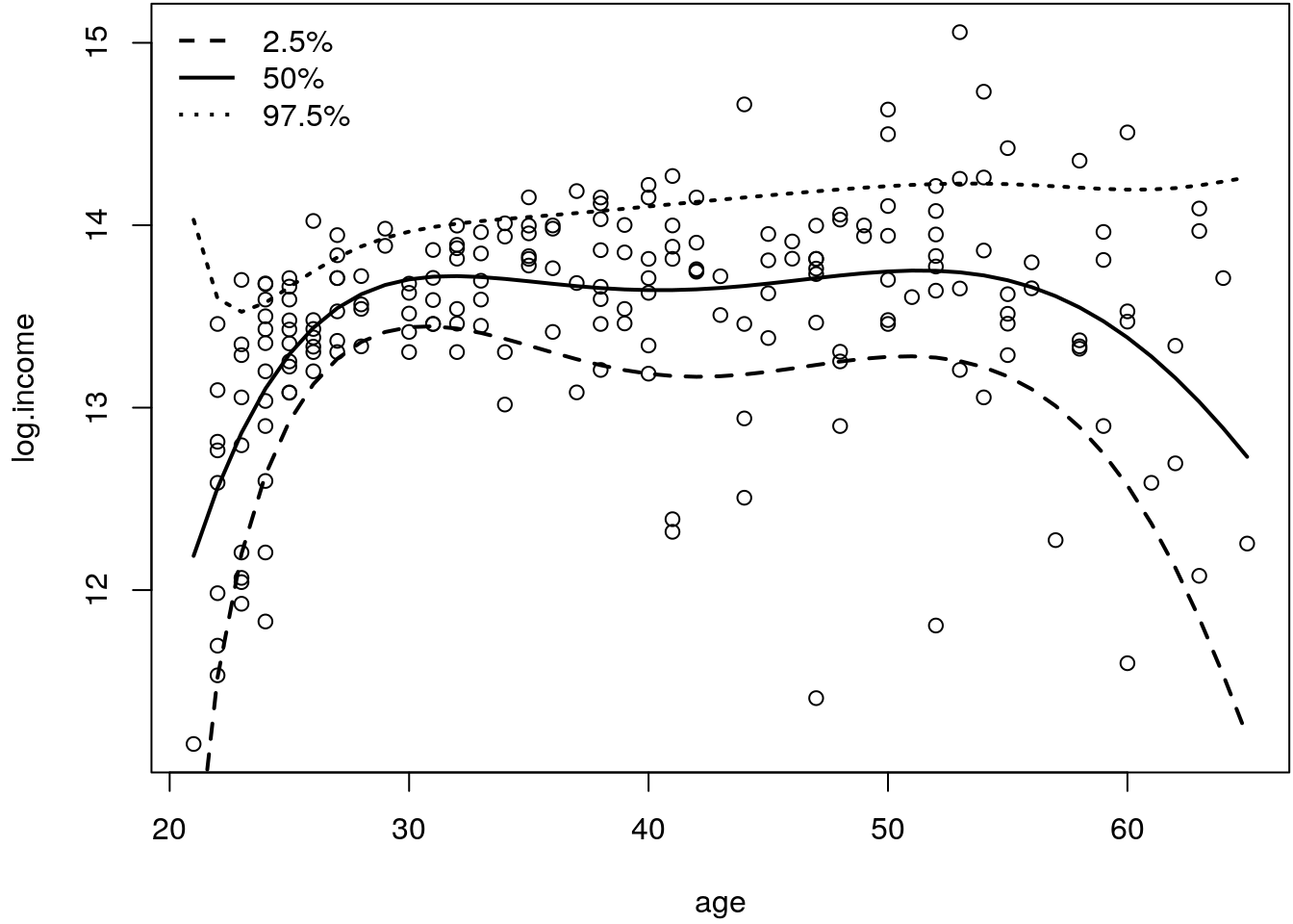
The plot suggests that we could capture the changing variance reasonably well, however, for, e.g., the top 97.5% quantile we first see a decrease in log income, which is not plausible. Hence, this seems to be an artifact of the model, which can happen for extreme values of the distribution using the two-step estimation approach. Especially in such situations it may be better to model these quantiles directly.
4.1 Quantiles
To understand the concept of quantile regression it is good to review quantiles in general. The theoretical quantiles \(q_{\tau}\), \(\tau \in (0,1)\), of a random variable \(y\) are defined by \[ P(y \leq q_{\tau}) \geq \tau \,\, \text{and} \,\, P(y \geq q_{\tau}) \geq 1 - \tau, \] i.e., the probability of observing a value below (above) \(q_{\tau}\) is at least \(\tau\) (and \(1 - \tau\), respectively).
Using this concept, empirical quantiles can be estimated by \[ \frac{1}{n} \sum_{i = 1}^n I(y_i \leq \hat{q}_{\tau}) \geq \tau \,\, \text{and} \,\, \frac{1}{n} \sum_{i = 1}^n I(y_i \geq \hat{q}_{\tau}) \geq 1 - \tau, \] where \(I( \cdot )\) is the indicator function. Hence, the fraction of observations that are below and above the quantile \(\hat{q}_{\tau}\) is computed and compared to \(\tau\). To introduce quantile regression models it is better to use the equivalent definition \[ \hat{q}_{\tau} = \underset{q}{\text{arg min}} \sum_{i=1}^n w_{\tau}(y_i, q)|y_i - q|, \] with \[ w_{\tau}(y, q) = \begin{cases} 1 - \tau & y < q \\ 0 & y = q \\ \tau & y > q, \end{cases} \] which is simply a weighted sum of absolute deviations. Let’s try this objective function, the following function illustrates the estimation of the empirical quantiles.
## Function to estimate quantiles from a numeric vector.
quantile2 <- function(x, probs = seq(0, 1, 0.25), ...) {
  ## Number of observations.
  n <- length(x)

  ## Objective to estimate quantile q.
  objfun <- function(q, tau) {
    w <- rep(1 - tau, n)
    w[x == q] <- 0
    w[x > q] <- tau
    sum(w * abs(x - q))
  }

  ## Estimate all quantiles.
  q <- list()
  for(tau in probs)
    q[[paste0(tau*100, "%")]] <- optimize(objfun, tau = tau, interval = range(x))$minimum

  ## Return estimated quantiles.
  return(unlist(q))
}

## Compute quantiles.
quantile2(age.income$log.income)
## 0% 25% 50% 75% 100%
## 11.15636 13.30470 13.60598 13.87381 15.05813## Compare to base R quantile() function.
quantile(age.income$log.income)## 0% 25% 50% 75% 100%
## 11.1563 13.3047 13.6060 13.8738 15.0582The two functions return the same quantiles. Note that differences might
occur due to the optimization algorithm in quantiles2(), quantiles are usually computed
much faster using a quicksort algorithm.
4.2 Estimation
Understanding the computation of the empirical quantiles is very helpful for setting up the complete quantile regression algorithm. Instead of one quantile \(q_{\tau}\) we specify the minimization problem from the last section in terms of regression coefficients \(\boldsymbol{\beta}_{\tau}\) with \[ \hat{\boldsymbol{\beta}}_{\tau} = \underset{\boldsymbol{\beta}}{\text{arg min}} \sum_{i=1}^n w_{\tau}(y_i, \eta_{i\tau}(\boldsymbol{\beta})) |y_i - \eta_{i\tau}(\boldsymbol{\beta})| \] and \[ \eta_{i\tau}(\boldsymbol{\beta}) = \mathbf{x}_i^{\top}\boldsymbol{\beta}. \] Hence, we simply replace the quantile \(q_{\tau}\) by the complete linear predictor and specify \[ w_{\tau}(y_i, \eta_{i\tau}(\boldsymbol{\beta})) = \begin{cases} 1 - \tau & y_i < \eta_{i\tau}(\boldsymbol{\beta}) \\ 0 & y_i = \eta_{i\tau}(\boldsymbol{\beta}) \\ \tau & y_i > \eta_{i\tau}(\boldsymbol{\beta}). \end{cases} \] For estimation it is useful to write the minimization problem using the check function \(\rho_{\tau}( \cdot )\) with \[ \hat{\boldsymbol{\beta}}_{\tau} = \underset{\boldsymbol{\beta}}{\text{arg min}} \sum_{i=1}^n \rho_{\tau}(y_i - \eta_{i\tau}(\boldsymbol{\beta})), \] with \[ \rho_{\tau}(u) = u(\tau - I(u < 0)) \] and indicator function \(I( \cdot )\). To compute \(\hat{\boldsymbol{\beta}}_{\tau}\) it would be nice if we could find a solution similar as in the linear regression model, however, this is actually not possible because the check function \(\rho_{\tau}( \cdot )\) is not differentiable at \(0\). Therefore, estimation algorithms usually rely on linear programming solutions. However, to illustrate the implementation we use a smooth and differentiable approximation of the check function (Zheng 2011) \[ S_{\tau, \alpha}(u) = \tau u + \alpha \log\left(1 + \exp\left(-\frac{x}{\alpha}\right)\right). \]
## The check function.
rho <- function(u, tau = 0.5) {
  u * (tau - 1 * (u < 0))
}

## Smooth version of check function.
S <- function(u, tau = 0.5, alpha = 0.005) {
  tau * u + alpha * log(1 + exp(-u / alpha))
}

## Compare.
par(mar = c(4.1, 4.1, 0.1, 0.1))
curve(rho, -0.1, 0.1, col = 2, lwd = 2)
curve(S, -0.1, 0.1, col = 1, lwd = 2, add = TRUE)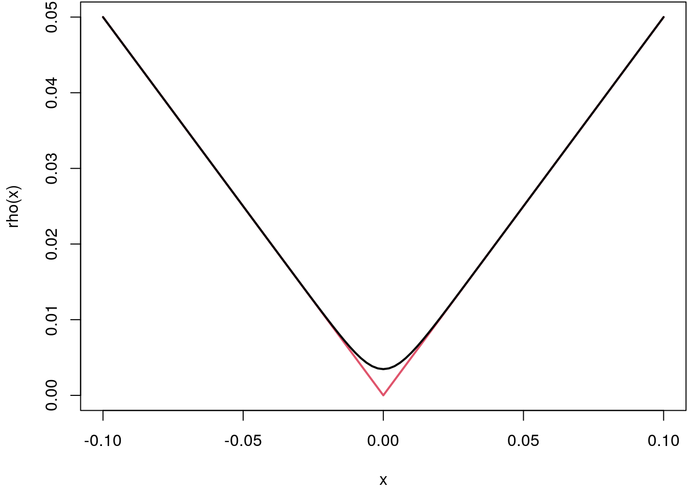
The smooth approximation is differentiable and convex, the smaller the parameter \(\alpha\), the sharper is the kink and therefore the better the approximation to the original check function.
We can hence use the smooth approximation for minimizing the objective function with
gradient based optimization functions as implemented in function optim(). The following
code is a bit more advanced, but it illustrates well how to set up linear quantile
regression with just a couple of lines of code. We re-estimate the log income model
again and compare to the two-step heteroskedastic model from the introduction above.
## Quantile regression model fitting engine
## using approximate check function.
qlm <- function(formula, data = NULL, tau = 0.5, alpha = 0.005, ...)
{
  ## Step 1, initial linear model.
  b <- lm(formula, data = data, ...)

  ## Extract the design matrix and the response
  X <- model.matrix(b)
  y <- model.response(model.frame(b))
  n <- length(y)

  ## The objective function to minimize.
  objfun <- function(beta, tau) {
    eta <- X %*% beta
    sum(S(y - eta, tau, alpha))
  }

  ## Estimate models for all quantiles.
  beta <- list()
  tau <- sort(tau)
  start <- coef(b)

  for(j in tau) {
    opt <- optim(start, fn = objfun, tau = j,
      method = "BFGS", control = list(maxit = 1e+08))
    beta[[paste0(j * 100, "%")]] <- opt$par
    start <- opt$par
  }

  ## Create matrix of coefficients.
  b$coefficients <- do.call("cbind", beta)

  ## Add the function call.
  b$call <- match.call()

  ## Assign a new class to implement some methods,
  ## e.g., predict().
  class(b) <- c("qlm", "lm")

  return(b)
}

## A simplified predict method, mainly copied from predict.lm().
predict.qlm <- function(object, newdata) {
  ## All we need for prediction is the new design matrix.
  class(object) <- "lm"
  tt <- terms(object)
  if(missing(newdata) || is.null(newdata)) {
    X <- model.matrix(object)
  } else {
    Terms <- delete.response(tt)
    m <- model.frame(Terms, newdata, xlev = object$xlevels)
    if(!is.null(cl <- attr(Terms, "dataClasses")))
      .checkMFClasses(cl, m)
    X <- model.matrix(Terms, m, contrasts.arg = object$contrasts)
  }

  ## Compute predictions.
  p <- list()
  for(j in colnames(object$coefficients))
    p[[j]] <- X %*% object$coefficients[, j]
  p <- as.data.frame(p)
  names(p) <- colnames(object$coefficients)

  return(p)
}

## Set quantiles for estimation.
tau <- c(0.025, 0.5, 0.975)

## Estimate models.
b <- qlm(log.income ~ poly(age, 5), data = age.income, tau = tau)

## Predict.
fit <- predict(b)

## And plot.
par(mar = c(4.1, 4.1, 0.1, 0.1))
plot(log.income ~ age, data = age.income)
matplot(age.income$age, fit, type = "l", lty = c(2, 1, 3), col = 1, lwd = 2, add = TRUE)
legend("topleft", paste0(tau*100, "%"), lwd = 2, lty = c(2, 1, 3), bty = "n")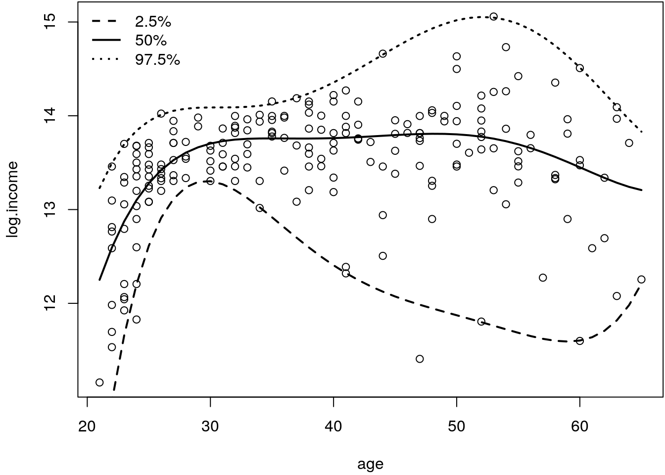
The estimate extreme quantiles (\(2.5\)% and \(97.5\)%) now look much more reasonable than in the two-step approach from the above. The estimated \(97.5\)% quantile is now increasing for age below \(30\) years, which was not the case before. Moreover, the extreme quantiles really represent the relationship of age and \(2.5\)% lowest and \(97.5\)% highest incomes.
Note that a much more efficient implementation of quantile regression is provdided in the quantreg package (Koenker 2020). We can estimate the model parameters including confidence intervals by
## Load the package
library("quantreg")
## Loading required package: SparseM##
## Attaching package: 'SparseM'## The following object is masked from 'package:base':
##
## backsolve## Estimate model.
m <- rq(log.income ~ poly(age, 5), data = age.income, tau = tau)
## Print model summary.
summary(m)## Warning in rq.fit.br(x, y, tau = tau, ci = TRUE, ...): Solution may be nonunique
## Warning in rq.fit.br(x, y, tau = tau, ci = TRUE, ...): Solution may be nonunique##
## Call: rq(formula = log.income ~ poly(age, 5), tau = tau, data = age.income)
##
## tau: [1] 0.025
##
## Coefficients:
## coefficients lower bd upper bd
## (Intercept) 1.229017e+01 1.208654e+01 1.237860e+01
## poly(age, 5)1 -3.510350e+00 -1.797693e+308 9.425000e-01
## poly(age, 5)2 -4.046730e+00 -1.797693e+308 -6.012200e-01
## poly(age, 5)3 6.086920e+00 -1.797693e+308 9.096200e+00
## poly(age, 5)4 -3.357830e+00 -1.870518e+01 -8.401300e-01
## poly(age, 5)5 2.065360e+00 -5.297700e+00 2.467680e+00
##
## Call: rq(formula = log.income ~ poly(age, 5), tau = tau, data = age.income)
##
## tau: [1] 0.5
##
## Coefficients:
## coefficients lower bd upper bd
## (Intercept) 13.55510 13.47230 13.60755
## poly(age, 5)1 2.38143 0.57910 3.24463
## poly(age, 5)2 -3.75685 -5.40169 -2.52316
## poly(age, 5)3 1.12854 -0.43444 2.45536
## poly(age, 5)4 -1.30394 -2.76422 -0.20460
## poly(age, 5)5 0.72446 -0.51708 2.22152
##
## Call: rq(formula = log.income ~ poly(age, 5), tau = tau, data = age.income)
##
## tau: [1] 0.975
##
## Coefficients:
## coefficients lower bd upper bd
## (Intercept) 1.432694e+01 1.418517e+01 1.433349e+01
## poly(age, 5)1 5.145300e+00 3.233640e+00 1.797693e+308
## poly(age, 5)2 -2.492310e+00 -2.801910e+00 1.797693e+308
## poly(age, 5)3 -2.181530e+00 -2.557230e+00 1.797693e+308
## poly(age, 5)4 -1.609020e+00 -2.948840e+00 2.421700e+00
## poly(age, 5)5 1.206760e+00 -1.790270e+00 2.516600e+00and again visualize with
## Compute predictions.
fit2 <- predict(m)

## Plot.
par(mar = c(4.1, 4.1, 0.1, 0.1))
plot(log.income ~ age, data = age.income)
matplot(age.income$age, fit, type = "l", lty = c(2, 1, 3), col = 1, lwd = 2, add = TRUE)
matplot(age.income$age, fit2, type = "l", lty = c(2, 1, 3), col = 2, lwd = 2, add = TRUE)
legend("topleft", paste0(tau*100, "%"), lwd = 2, lty = c(2, 1, 3), bty = "n")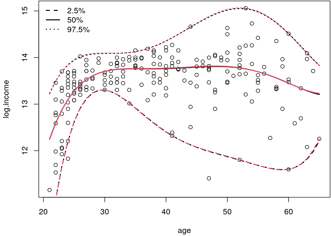
Which produces quite similar fits as can be seen by the mostly overlapping estimated curves for the three quantiles.
MunichRent data and estimate the following linear
quantile regression model
\[
\texttt{rent}_i = \beta_0 + f(\texttt{area}_i) \cdot \beta_1 + \varepsilon_i,
\]
for \(\tau = 0.01, 0.1, 0.2, \ldots, 0.8, 0.9, 0.99\) and function \(f( \cdot )\) is
an orthogonal polynomial of degree \(3\). Compare the estimated quantiles with the two-step
heteroskedastic Weighted least squares algorithm implemented in function hetlm().
For estimation of the quantile regression models use the rq() function of the
quantreg package.
First, we load the required package and data.
library("quantreg")
load("data/MunichRent.rda")
Set up the vector of quantiles.
tau <- c(0.01, seq(0.1, 0.9, by = 0.1), 0.99)Estimate quantile regression models
b1 <- rq(rent ~ poly(area, 3), data = MunichRent, tau = tau)and the heteroskedastic linear model
b2 <- hetlm(rent ~ poly(area, 3), data = MunichRent)Compute fitted quantiles for both
## Quantile regression fit.
fit1 <- predict(b1)

## Heteroskedastic LM fit.
p2 <- predict(b2$mean)
sigma2 <- exp(predict(b2$variance))
fit2 <- matrix(NA, nrow = length(p2), ncol = length(tau))
for(j in seq_along(tau)) {
  fit2[, j] <- p2 + qnorm(tau[j], mean = 0, sd = sqrt(sigma2))
}

## Compare.
par(mfrow = c(1, 2))

ylim <- range(c(MunichRent$rent, fit1, fit2))

plot(rent ~ area, data = MunichRent, col = rgb(0.1, 0.1, 0.1, alpha = 0.4),
  main = "Quantile regression", ylim = ylim)
i <- order(MunichRent$area)
matplot(MunichRent$area[i], fit1[i, ], type = "l", lty = 1,
  lwd = 2, col = 4, add = TRUE)

plot(rent ~ area, data = MunichRent, col = rgb(0.1, 0.1, 0.1, alpha = 0.4),
  main = "Heteroskedastic LM", ylim = ylim)
i <- order(MunichRent$area)
matplot(MunichRent$area[i], fit2[i, ], type = "l", lty = 1,
  col = 4, lwd = 2, add = TRUE)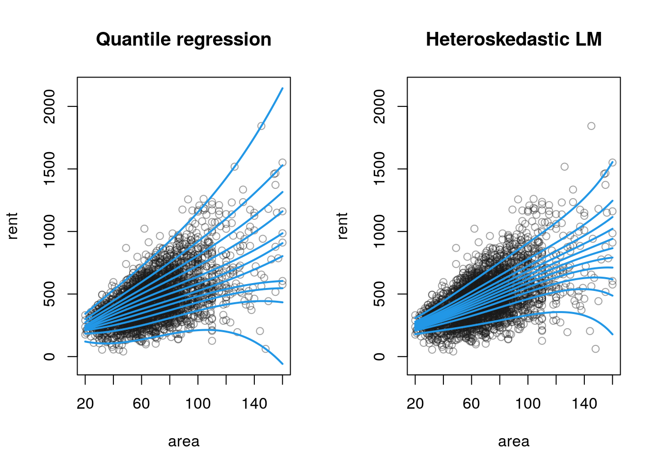
The plots show that the estimated quantiles are quite different for both methods. The more extreme quantiles of the heteroskedastic linear model are largely underestimated and do not really represent the correct fractions of the rent.