Chapter 2 Model choice criteria

One widely used criteria for model choice is the adjusted R^2, see section Goodness-of-fit. However, the adjusted \(R^2\) has a couple limitations. Probably the largest downside is that the penalty that should adjust for newly included covariates is too weak, i.e., models tend to overfit the data. We therefore recommend not to use the adjusted \(R^2\) as a model selection tool. In the following we describe five other commonly used information criteria.

2.1 Extra sum of squares

We often need to compare two or more models. E.g., let’s look the UsedCars data set. A simple model to explain the price of a car is \[ \texttt{price}_i = \beta_0 + \beta_1\texttt{age}_i + \varepsilon_i. \] However, when looking at the scatterplot of the data

load("data/UsedCars.rda")

par(mar = c(4.1, 4.1, 0.1, 0.1))
plot(price ~ age, data = UsedCars)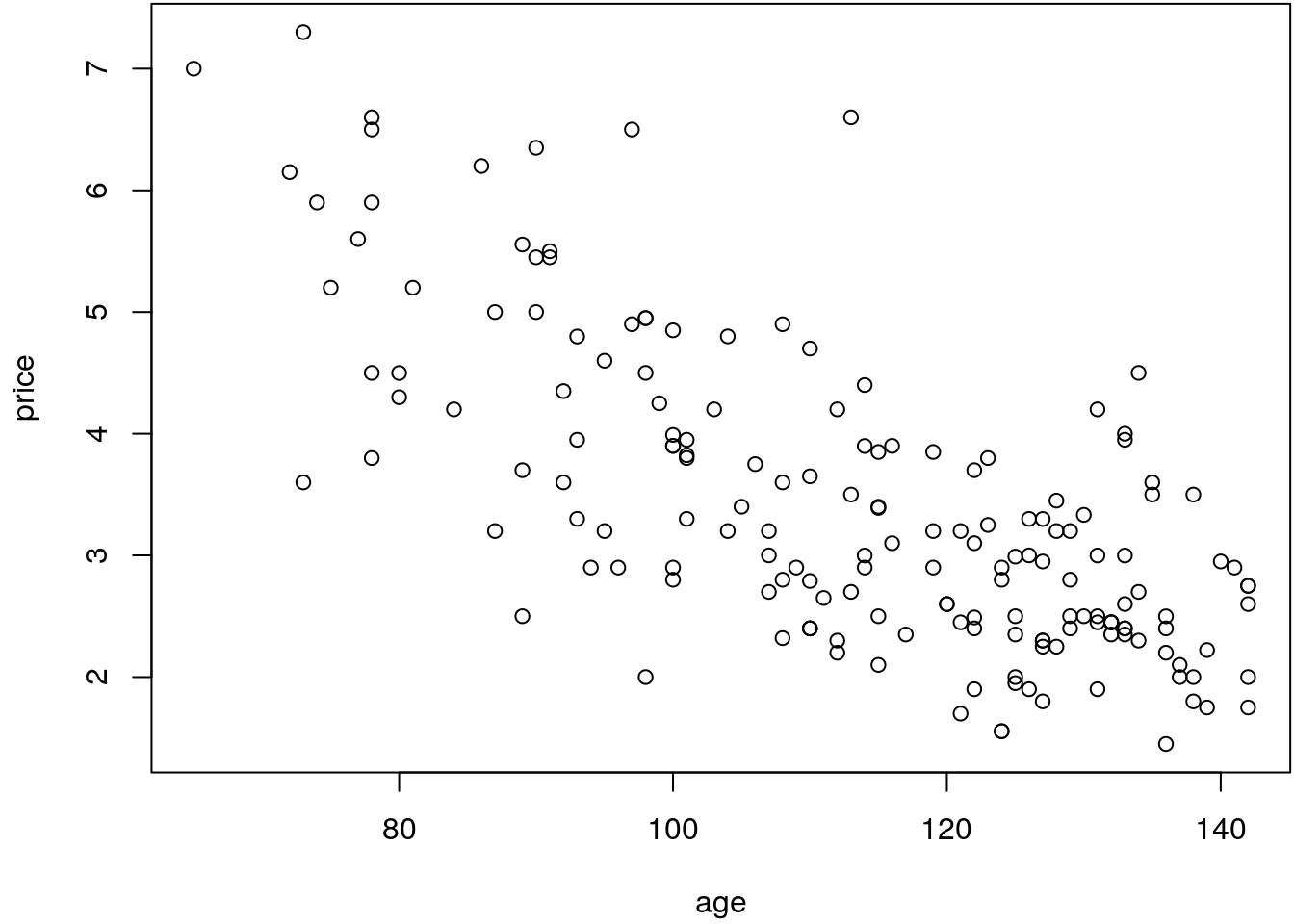

It seems like that the relationship is slightly nonlinear, so a straight line model might not be appropriate.

Now consider a quadratic model \[ \texttt{price}_i = \beta_0 + \beta_1\texttt{age}_i + \beta_2\texttt{age}_i^2 + \varepsilon_i. \] and estimate both models.

b1 <- lm(price ~ age, data = UsedCars)
b2 <- lm(price ~ age + I(age^2), data = UsedCars)

## Plot the fitted lines.
i <- order(UsedCars$age)
fit1 <- fitted(b1)
fit2 <- fitted(b2)

par(mar = c(4.1, 4.1, 0.1, 0.1))
plot(price ~ age, data = UsedCars)
lines(fit1[i] ~ UsedCars$age[i], col = 1, lwd = 2)
lines(fit2[i] ~ UsedCars$age[i], col = 2, lwd = 2)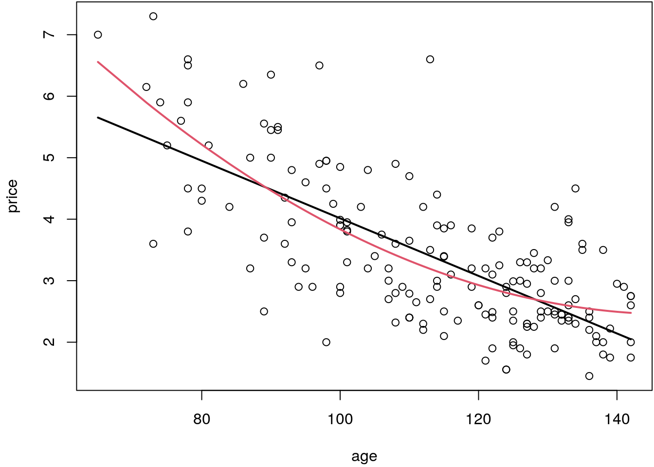

The quadratic fit appears to be better, but is this just due to random variation or is there really a curvature that requires an alternative to the straight line model?

We can address this question by testing \[ H_0: \beta_2 = 0 \,\, \text{versus} \,\, H_1: \beta_2 \not= 0. \]
The least squares estimator minimizes \(RSS = \boldsymbol{\varepsilon}^\top\boldsymbol{\varepsilon}\), which is a cursory measure of the quality of the fit. If one model fits better than the other, then this difference in fit should be evident in the \(RSS\) values.
The extra sum of squares is \(ExtraSS \equiv RSS_{\text{linear}} - RSS_{\text{quadratic}}\), \ or more general \[ ExtraSS \equiv RSS_{\text{smaller}} - RSS_{\text{larger}}. \]

The extra sum of squares can be used to test the larger versus the smaller models. The null hypothesis is that the smaller models fit the data.

Let \(p_{\text{smaller}}\) and \(p_{\text{larger}}\) be the number of parameters of the respective models. The \(F\)-test statistic is \[ F \equiv \frac{ExtraSS / (p_{\text{larger}} - p_{\text{smaller}})}{\hat{\sigma}_{\text{larger}}^2}. \] Under the null hypothesis and the normality assumption, \(F\) has a \(F\)-distribution with \(p_{\text{larger}} - p_{\text{smaller}}\) and \(n - p_{\text{larger}}\) degrees of freedom. The \(F\)-statistic compares the improvement per parameter to the data variability. The null hypothesis should be rejected when \(F\) is large.

An \(\alpha\)-level test is obtained by rejecting the null hypothesis when \(F\) exceeds the \(1 - \alpha\) quantile of the \(F\)-distribution with \(p_{\text{larger}} - p_{\text{smaller}}\) and \(n - p_{\text{larger}}\) degrees of freedom.

Let’s test this on the UsedCars data:

n <- nrow(UsedCars)
e1 <- residuals(b1); e2 <- residuals(b2)
RSS1 <- t(e1) %*% e1; RSS2 <- t(e2) %*% e2;
p1 <- length(coef(b1)); p2 <- length(coef(b2))
sigma2 <- drop(RSS2/b2$df.residual)
F <- drop(((RSS1 - RSS2) / (p2 - p1)) / sigma2)
F

## [1] 10.99765

pvalue <- 1 - pf(F, p2 - p1, n - p2)
pvalue

## [1] 0.001116711

The small P-value suggests that the model with the quadratic term covariate age fits better. In this setting the test seems to give a plausible result. However, for more complex models including more covariates this strategy has a severe problem:

Hypothesis testing is “biased” towards the null hypothesis in that we retain the null unless there is strong evidence to the contrary.
When we want to compare two models, we often want to treat them on an equal footing rather than accepting one unless there is strong evidence against it.
One alternative is to try to find the model that gets as close as possible to the true model.
We can attempt to find the model which does the best job of predicting \(E(y_i)\).

2.2 Cross validation

In many applications, a large (potentially enormous) number of candidate predictor variables is available, and we face the challenge and decision as to which of these variables to include in the regression model.

As a typical example, take the MunichRent data with approximately 200 variables that are collected through a questionnaire. The following are two naive (but often practiced) approaches to the model selection problem:

Strategy 1: Estimate the most complex model which includes all available covariates.
Strategy 2: First estimate a model with all variables. Then, remove all insignificant variables from the model.

Both strategies will not result in a very good predictive model. This can be shown easily, e.g., using polynomial regression we estimate the model \[ \texttt{rentsqm}_i = \beta_0 + f(\texttt{area}_i) + \varepsilon_i, \] where function \(f( \cdot )\) is a polynomial of degree \(l\). Now, we split the MunichRent data randomly in 80% training data and 20% testing data:

## Load the data.
load("data/MunichRent.rda")

## Set the seed for reproducibility.
set.seed(456)

## Add indicator variable to split the data set.
MunichRent$id <- sample(1:2, size = nrow(MunichRent), replace = TRUE, prob = c(0.8, 0.2))

Then, we estimate a number of models where we increase the degree of the polynomial. We use the full data set as well as the reduced data set with 80% of the observations. Then, we calculate the mean squared error (MSE) for the full data set, and the MSE on the 20% out-of-sample data set.

mse1 <- mse2 <- NULL
degrees <- 1:20
for(l in degrees) {
  b1 <- lm(rentsqm ~ poly(area, degree = l), data = MunichRent)
  b2 <- lm(rentsqm ~ poly(area, degree = l), data = MunichRent, subset = id == 1)

  mse1 <- c(mse1, with(MunichRent, mean((rentsqm - fitted(b1))^2)))

  p <- predict(b2, newdata = subset(MunichRent, id == 2))
  mse2 <- c(mse2, with(MunichRent, mean((rentsqm[id == 2] - p)^2)))
}

The effect of increasing the number of covariates using polynomial regression can then be visualized with:

par(mfrow = c(1, 2), mar = c(4.1, 4.1, 0.1, 0.5))
matplot(degrees, cbind(log(mse1), log(mse2)), type = "l",
  xlab = "Degree", ylab = "log(MSE)", col = 1:2, lwd = 2, lty = 1)
legend("topright", c("Full data", "Subset"),
  lty = 1, col = 1:2, lwd = 2, bty = "n")
l1 <- which.min(mse1)
l2 <- which.min(mse2)
print(l1)

## [1] 20

print(l2)

## [1] 6

b1 <- lm(rentsqm ~ poly(area, degree = l1), data = MunichRent)
b2 <- lm(rentsqm ~ poly(area, degree = l2), data = MunichRent)
plot(rentsqm ~ area, data = MunichRent,
  col = rgb(0.1, 0.1, 0.1, alpha = 0.3), cex = 0.3)
with(subset(MunichRent, id == 1), points(area, rentsqm,
  col = rgb(0.7, 0.1, 0.1, alpha = 0.3), pch = 16, cex = 0.3))
i <- order(MunichRent$area)
lines(fitted(b1)[i] ~ area[i], data = MunichRent, lwd = 2)
lines(fitted(b2)[i] ~ area[i], data = MunichRent, lwd = 2, col = 2)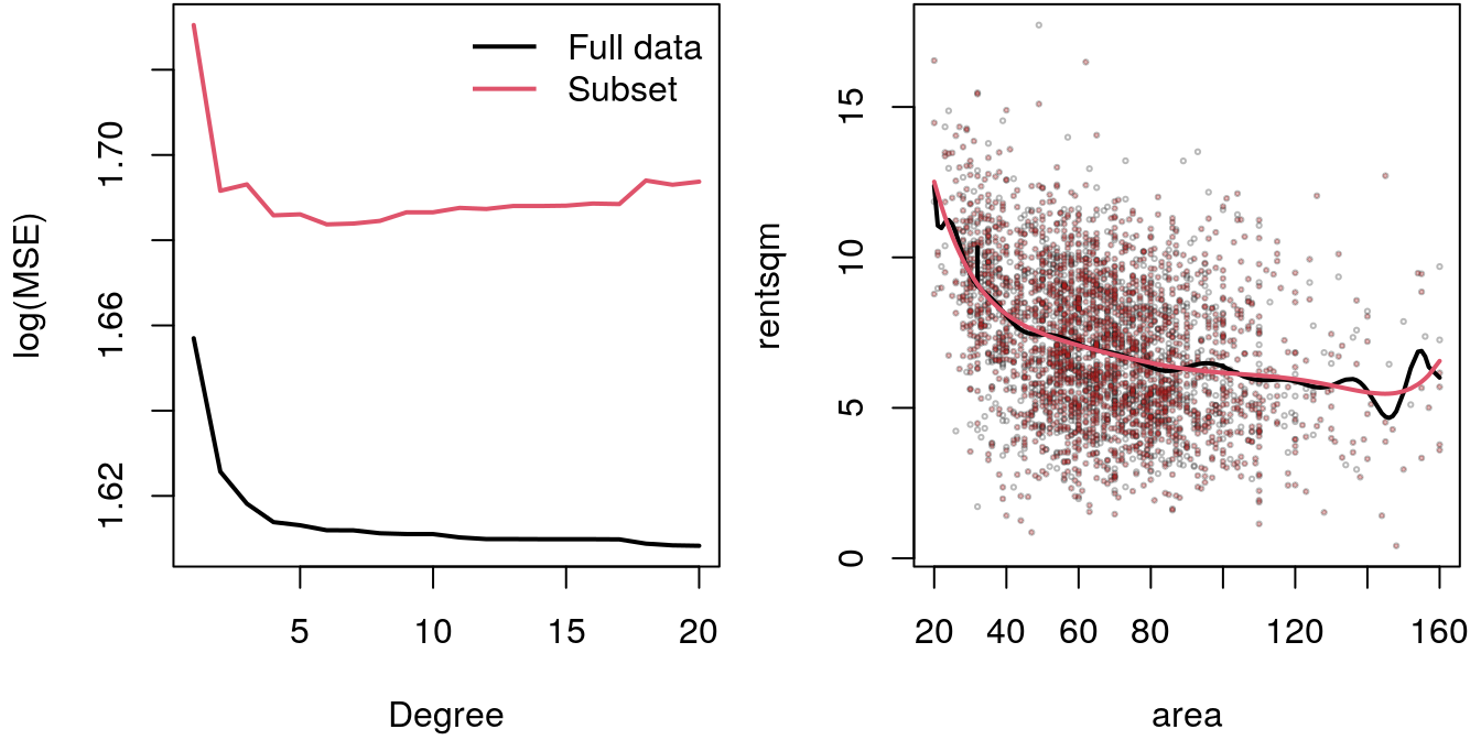

Here, the final degree of the polynomial using the full data set is 20, the degree of the polynomial that is searched using the 20% out-of-sample data is only 6. The effect is clear, when looking at the MSE using the full data set, the MSE get’s smaller and smaller the higher the degree of the polynomial is (the higher the number of covariates so to say). If we evaluate the MSE on an out-of-sample data set, we first obtain a decrease but then after a couple of steps the MSE increases. This means that we run into the problem of overfitting quite quickly, if we do not optimize the model accordingly. The overfitting effect is visualized in the right panel. The black line using a degree 20 polynomial is very wiggly and seems to interpolate the data quite a bit. The red line represents the 6 degree polynomial and is much smoother.

In summary, cross validation (CV) is a very useful tool for creating models with great predictive performance. In a real modelling situation, the cross validation step presented above is done a number of times with randomly selected subsets of the data. In each step the optimum set of variables (or hyperparameters) is selected. The average result can then be used to set up a final model, or through aggregation of the single model predictions. So, cross validation is based on the following general principle:

Partition the data set into \(r\) subsets \(1, \dots, r\), of similar size.
Start with the first data set as validation set and use the combined remaining \(r-1\) data sets for parameter estimation. Based on the estimates, obtain predictions for the validation set and determine the sum of the squared prediction errors.
Cycle through the partitions using the second, third, up to the \(r\)th data set as validation sample, and all other data sets for estimation. Determine the sum of squared prediction errors.

2.3 Leave one out cross validation

The cross validation procedure of the last section cannot be done in all situations, e.g., if the number of observations is not large enough to find suitable subsets. Therefore, we need other tools that account for this but still give reasonable results in a model selection situation.

As shown above, the \(RSS\) of a model is a measure of predictive ability, however, it is not satisfactory as a model selector. The problem is that the model with the largest number of parameters and containing the other models as special cases always has the smallest \(RSS\).

Now consider the model \(y_i = f(x_{i1}, \dots, x_{ik}) + \varepsilon_i\). Ideally, it would be good to choose a model so that the estimate \(\hat{f}\) is as close as possible to \(f\). A suitable criterion might be \[ M = \frac{1}{n} \sum_{i = 1}^n \left(\hat{f}_i - f_i\right)^2. \] Since \(f\) is unknown, \(M\) cannot be computed directly, but it is possible to derive an estimate of \(E(M) + \sigma^2\).

Let \(\hat{f}^{(k)}\) be the model fitted to all data except \(y_k\), the ordinary cross validation score is \[ V_o = \frac{1}{n} \sum_{i = 1}^n \left(\hat{f}_i^{(k)} - y_i\right)^2. \] Substituting \(y_i = f_i + \varepsilon_i\), \[\begin{align} V_o &= \frac{1}{n} \sum_{i = 1}^n \left(\hat{f}_i^{(k)} - f_i - \varepsilon_i\right)^2 \\ &= \frac{1}{n} \sum_{i = 1}^n \left(\hat{f}_i^{(k)} - f_i\right)^2 - \left(\hat{f}_i^{(k)} - f_i\right)\varepsilon_i + \varepsilon_i^2. \end{align}\] Since \(E(\varepsilon_i) = 0\) and \(\varepsilon_i\) and \(\hat{f}^{(k)}\) are independent, we get \[ E(V_o) = \frac{1}{n} E\left(\sum_{i = 1}^n \left(\hat{f}_i^{(k)} - f_i\right)^2\right) + \sigma^2. \] Now, in the large limit, \(\hat{f}^{(k)} \approx \hat{f}\), so \(E(V_o) \approx E(M) + \sigma^2\), hence choosing the model that minimizes \(V_o\) is a reasonable approach if the ideal would be to minimize \(M\).

Note that it is computationally inefficient to compute the cross validation score the way it is done in the above. A more efficient way is given by \[ V_o = \frac{n \sum_{i = 1}^n (y_i - \hat{f}_i)^2}{[trace(\mathbf{I} - \mathbf{H})]^2}, \] which is also called the generalized cross validation (GCV) score and matrix \(\mathbf{H}\) is the hat-matrix, see section Least squares.

Exercise 2.1 Set up a new function that computes the GCV criterion and has the argument

GCV(object)

where object is an fitted model object as returned from function lm(). Use the function to select the best fitting polynomial in the MunichRent data example, i.e., fit polynomial models \[ \texttt{rentsqm}_i = \beta_0 + f(\texttt{area}_i) + \varepsilon_i, \] where function \(f( \cdot )\) is a polynomial of degree \(l\). Compare the result to the cross validation exercise from the above.

The data is loaded with

load("data/MunichRent.rda")

The GCV() function can be set up with

GCV <- function(object, ...) {
  e <- residuals(object)
  n <- length(e)
  RSS <- crossprod(e)
  trH <- sum(influence(object)$hat[1:n])
  drop(n * RSS / (n - trH)^2)
}

Now, we fit a number of polynomial models and compute the GCV score for each model.

degree <- 1:20
gcv <- rep(0, length(degree))
for(i in seq_along(degree)) {
  b <- lm(rentsqm ~ poly(area, degree[i]), data = MunichRent)
  gcv[i] <- GCV(b)
}

## Extract model with minimum GCV score.
i <- which.min(gcv)
print(gcv[i])

## [1] 5.035375

print(degree[i])

## [1] 6

b <- lm(rentsqm ~ poly(area, degree[i]), data = MunichRent)

## Plot.
par(mfrow = c(1, 2), mar = c(4.1, 4.1, 0.5, 0.7))
plot(gcv ~ degree, type = "l")
abline(v = which.min(gcv), lty = 2, col = "lightgray") 
plot(rentsqm ~ area, data = MunichRent,
  col = rgb(0.1, 0.1, 0.1, alpha = 0.2), cex = 0.3)
i <- order(MunichRent$area)
p <- predict(b, interval = "confidence")
matplot(MunichRent$area[i], p[i, ], type = "l",
  lty = c(1, 2, 2), col = 2, add = TRUE, lwd = c(2, 1, 1))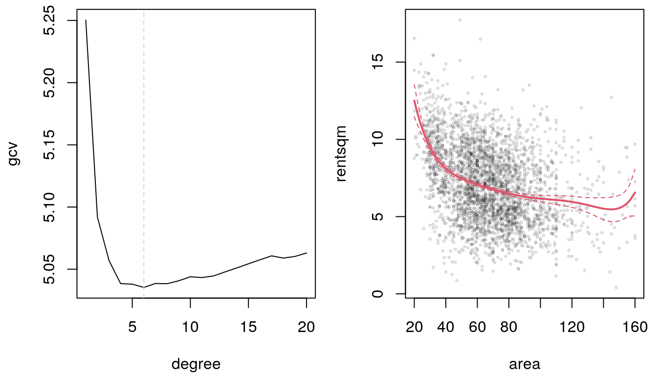

According the GCV criterion a polynomial model of degree 6 fits best. This finding is inline with the resulting degree of the polynomial in the cross validation exercise from the above. The estimated smooth effect of area seems fit the data quite well.

2.4 Akaike information criterion

The Akaike information criterion (AIC) is one of the most widely used criteria for model choice within the scope of likelihood-based inference.

In general, AIC is defined by \[ \text{AIC} = -2 \cdot \ell(\hat{\boldsymbol{\beta}}_M, \hat{\sigma}^2) + 2 \, (|M|+1), \] where \(\ell(\hat{\boldsymbol{\beta}}_M, \hat{\sigma}^2)\) is the maximum value of the log-likelihood. Smaller values of the AIC correspond to a better model fit.

Comparing two (or more) models, the difference of AIC values is considered to be “significant” if \[ |AIC(M_1) - AIC(M_2)| > 2. \]

The AIC of a model can be extracted using the generic function AIC().

2.5 Bayesian information criterion

The Bayesian information criterion (BIC) penalizes model complexity even more.

The BIC is defined by \[ \text{BIC} = -2 \cdot \ell(\hat{\boldsymbol{\beta}}_M, \hat{\sigma}^2) + \log(n) \, (|M| + 1). \] For \(\log(n) \geq 2 \Leftrightarrow n \geq 8\), the BIC clearly penalizes model complexity more than the \(AIC\).

The BIC of a model can be extracted using the generic function BIC().