Chapter 7 Exercises

7.1 Linear models

7.1.1 Speed and stopping distances of cars

Note, the example is taken from Wood (2006).

This exercise is about modelling the relationship between stopping distance of a car and its speed at the moment that the driver is signalled to stop. Data on this are provided in R data frame cars. The data can be loaded with

data("cars", package = "datasets")
print(head(cars))
##   speed dist
## 1     4    2
## 2     4   10
## 3     7    4
## 4     7   22
## 5     8   16
## 6     9   10

It takes a more or less fixed ‘reaction time’ for a driver to apply the car’s brakes, so that the car will travel a distance directly proportional to its speed before beginning to slow. A car’s kinetic energy is proportional to the square of its speed, but the brakes can only dissipate that energy, and slow the car, at a roughly constant rate per unit distance travelled: so we expect that once braking starts, the car will travel a distance proportional to the square of its initial speed, before stopping.

  1. Given the information provided above, fit a model of the form \[ \texttt{dist}_i = \beta_0 + \beta_1 \texttt{speed}_i + \beta_2 \texttt{speed}^2_i + \varepsilon_i \] to the data in cars, and from this starting model, select the most appropriate model for the data using both AIC, and hypothesis testing methods.
  2. From your selected model, estimate the average time that it takes a driver to apply the brakes (there are 5280 feet in a mile).
  3. When selecting between different polynomial models for a set of data, it is often claimed that one should not leave in higher powers of some continuous predictor, while removing lower powers of that predictor. Is this sensible?

7.1.2 Climate reconstruction data

The data set moberg2005 contains information on reconstructions of the average yearly temperature on the Northern hemisphere for the last 2000 years which allows us to study trends in the temperature evolution. For the following analyses, we assume that the average yearly temperature is normally distributed with a constant variance but time-dependent expectation, i.e. \[ \texttt{temperature} \sim \mathrm{N}(f(\texttt{time}), \sigma^2). \]

  1. Estimate a polynomial model for the temporal trend function.
  2. Search for the best fitting polynomial using the BIC() function.
  3. Visualize the best fitting model including the raw observations, the fitted line as well as estimated 95% confidence intervals.

7.1.3 Heteroskedasticity

Note, the data is taken from Wooldridge (2016).

The data set hprice.rds contains \(321\) observations of house prices in the US. Consider the following linear predictor \[ \texttt{price} = \beta_0 + f_1(\texttt{area}) + f_2(\texttt{age}) + f_3(\texttt{intst}), \] where each function \(f_j( \cdot )\) should be modeled using orthogonal polynomials of degree \(3\). Is there a heteroskedasticity problem? If yes, estimate a heteroskedasticity corrected model. What happens if you use log(price) as the dependent variable?

7.2 Semiparametric regression

7.2.1 Motorcycle accident data

For this exercise load the mcycle data set from the MASS package.

  1. According the AIC(), find the best fitting polynomial model.
  2. Compute the normalized residuals and check if they are in line with the assumptions of the linear regression model. Are there any outliers?
  3. Check for autocorrelation in the residuals using function acf().
  4. Now, set up a function tp() with arguments tp(z, degree = 3, knots = seq(min(z), max(z), length = 10)) that returns a design matrix of basis functions of a polynomial spline with truncated powers representation. Argument is the covariate used to set up the design matrix, degree is the maximum degree of the polynomial and knots are the knots that split up the range of z in intervals, default is 9 intervals with 10 equidistant knots.
  5. It is computationally inefficient to compute the (CV) score the way it is done in the slides. A more efficient way is given by \[ V_o = \frac{n \sum_{i = 1}^n (y_i - \hat{f}_i)^2}{[trace(\mathbf{I} - \mathbf{A})]^2}. \] which is also called the (GCV) score. Set up a new function GCV() that computes the GCV criterion and has the arguments GCV(y, Z) where y is the response and Z a design matrix that is used for estimating a linear model by ordinary least squares.
  6. From the code of 6., find a model using function tp() that best fits the mcycle data according the returned GCV criterion of function GCV() (try out different knot locations and degrees by hand).
  7. Finally, check if the best fitting spline model is better than the best fitting polynomial model of 1. according the GCV score.

7.2.2 Bike share data

Note, the data is taken from the UCI Machine Learning Repository.

Bike sharing systems help to make it easier to rent a bike. They automate the process of purchasing membership, renting and returning bikes through a network of kiosk locations across the city. Using these systems, people can borrow a bike in one place and return it to another if needed. For the system to work it is therefore important to know the demand for bikes at certain points in time. This exercise is about building a good predictive model for the demand for bikes.

The BikeShare.rda dataset contains a sample of 17389 days on which the amount of rented bicycles and weather data are recorded (Fanaee-T and Gama 2013). The data were collected between 2011 and 2012 and includes the following variables:

Variable Description
instant Record index.
dteday Date.
season Season (1: Winter, 2: Spring, 3: Summer, 4: Fall).
yr Year (0: 2011, 1: 2012).
mnth Month (1:12).
hr Hour (0:23).
holiday Weather day is holiday or not.
weekday Day of the week.
workingday If day is neither weekend nor holiday is 1, otherwise is 0.
weathersit 1: Clear, Few clouds, Partly cloudy, Partly cloudy; 2: Mist + Cloudy, Mist + Broken clouds, Mist + Few clouds, Mist; 3: Light Snow, Light Rain + Thunderstorm + Scattered clouds, Light Rain + Scattered clouds; 4: Heavy Rain + Ice Pallets + Thunderstorm + Mist, Snow + Fog.
temp Normalized temperature in Celsius.
atemp Normalized feeling temperature in Celsius.
hum Normalized humidity. The values are divided to 100 (max).
windspeed Normalized wind speed. The values are divided to 67 (max).
casual Count of casual users.
registered Count of registered users.
cnt Count of total rental bikes including both casual and registered.

Using the tools for semiparametric regression models as provided in the mgcv package, find the best model to explain the response cnt. Therefore, also keep in mind that the i.i.d. assumption is not fulfilled, since we are looking at time-series type data.

7.3 Bayesian models.

7.3.1 Slice sampling

Take a close look at the implementation of the slice sampler in section Slice MCMC. If we want to perform slice MCMC for models with more parameters, how does the implementation need to be changed? Try to adapt it and estimate a regression model using the following simulated data: \[ y = 1.2 + sin(x) + \varepsilon \] and \(\varepsilon \sim N(0, 0.3^2)\)

set.seed(123)

n <- 300

x <- runif(n, -2 * pi, 2 * pi)
y <- 1.2 + sin(x) + rnorm(n, sd = 0.3)

par(mar = c(4.1, 4.1, 0.1, 0.1))
plot(x, y)

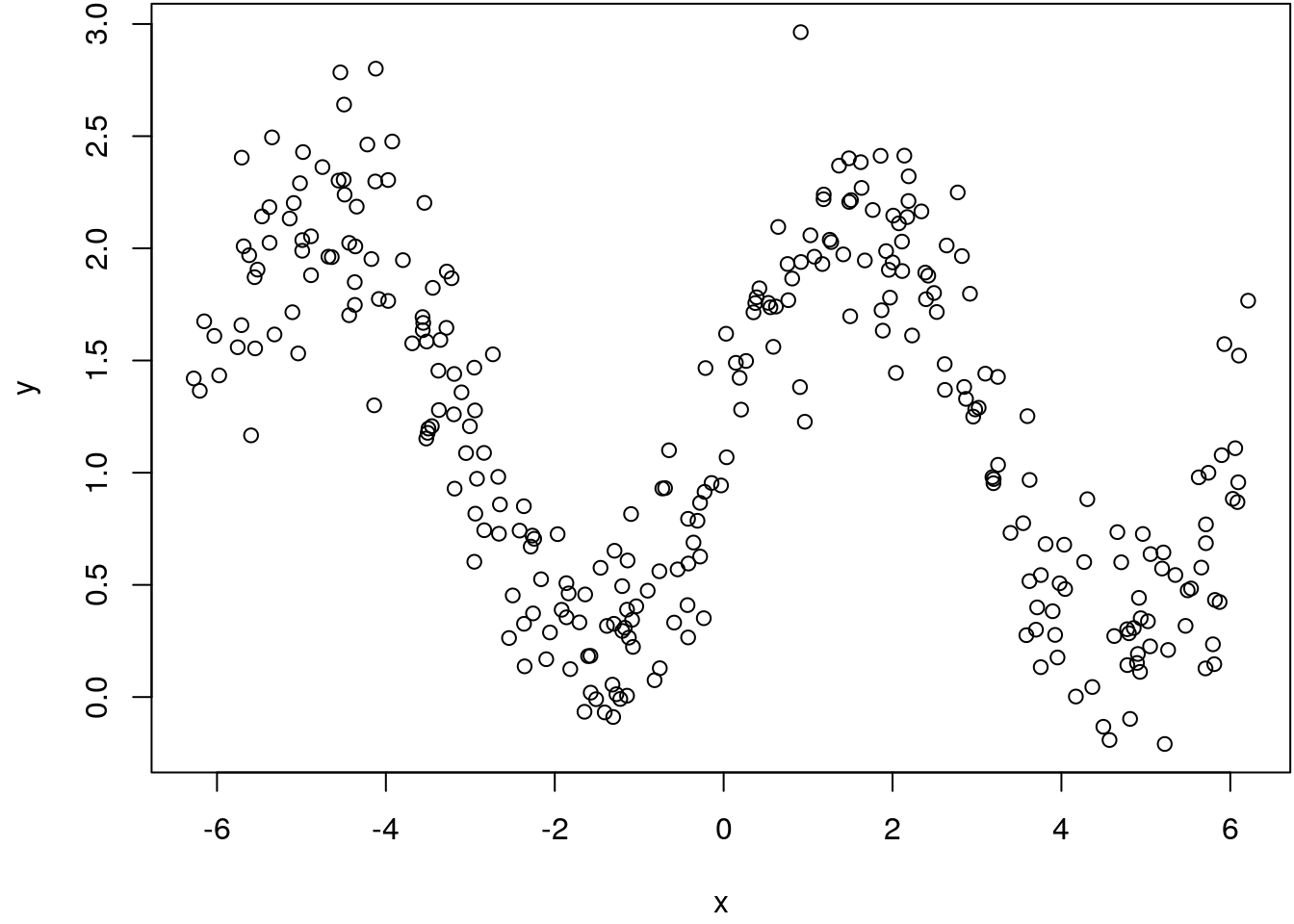
See also the Linear model example how the target posterior distribution is set up for the slice sampler.

7.4 Advanced modeling

7.4.1 Boston housing

A quite popular data set that has been used extensively throughout the literature to benchmark algorithms is the Boston Housing data set.

Harrison, D. and Rubinfeld, D.L. Hedonic Pices and the Demand for Clean Air, J. Environ. Economics & Management, 5, 81-102, 1978.

The data set is available in the mlbench package and can be load with

if(!require("mlbench")) {
  install.packages("mlbench")
}
## Loading required package: mlbench
data("BostonHousing2", package = "mlbench")

The data set consists of 506 observations and 19 variables.

print(head(BostonHousing2))
##         town tract      lon     lat medv cmedv    crim zn indus chas   nox
## 1     Nahant  2011 -70.9550 42.2550 24.0  24.0 0.00632 18  2.31    0 0.538
## 2 Swampscott  2021 -70.9500 42.2875 21.6  21.6 0.02731  0  7.07    0 0.469
## 3 Swampscott  2022 -70.9360 42.2830 34.7  34.7 0.02729  0  7.07    0 0.469
## 4 Marblehead  2031 -70.9280 42.2930 33.4  33.4 0.03237  0  2.18    0 0.458
## 5 Marblehead  2032 -70.9220 42.2980 36.2  36.2 0.06905  0  2.18    0 0.458
## 6 Marblehead  2033 -70.9165 42.3040 28.7  28.7 0.02985  0  2.18    0 0.458
##      rm  age    dis rad tax ptratio      b lstat
## 1 6.575 65.2 4.0900   1 296    15.3 396.90  4.98
## 2 6.421 78.9 4.9671   2 242    17.8 396.90  9.14
## 3 7.185 61.1 4.9671   2 242    17.8 392.83  4.03
## 4 6.998 45.8 6.0622   3 222    18.7 394.63  2.94
## 5 7.147 54.2 6.0622   3 222    18.7 396.90  5.33
## 6 6.430 58.7 6.0622   3 222    18.7 394.12  5.21

In this example, the aim is to model the corrected median value of owner-occupied homes using a smooth additive model. Therefore, split the data into a 80% training and 20% testing set with

set.seed(123)
id <- sample(1:2, size = nrow(BostonHousing2), replace = TRUE, prob = c(0.8, 0.2))
dtrain <- subset(BostonHousing2, id == 1)
dtest <- subset(BostonHousing2, id == 2)
print(nrow(dtrain))
## [1] 412
print(nrow(dtest))
## [1] 94

Using the methods from section linear models to smooth additive models, find a model that minimizes the out-of-sample MSE (data frame dtest) \[ \text{MSE} = \frac{1}{n} \sum_{i = 1}^n (\text{cmedv} - \widehat{\text{cmedv}})^2. \]

Visualize the estimated effects and interpret the results. Therefore, build a statistical report using Rmarkdown which also shows all the model building steps.

Demidenko, Eugene. 2016. “The p-Value You Can’t Buy.” The American Statistician 70 (1): 33–38. https://doi.org/10.1080/00031305.2015.1069760.
Fahrmeir, Ludwig, Thomas Kneib, Stefan Lang, and Brian Marx. 2013. Regression – Models, Methods and Applications. Berlin: Springer-Verlag.
Fanaee-T, Hadi, and Joao Gama. 2013. “Event Labeling Combining Ensemble Detectors and Background Knowledge.” Progress in Artificial Intelligence, 1–15. https://doi.org/10.1007/s13748-013-0040-3.
Fortran code by Alan Miller, Thomas Lumley based on. 2020. Leaps: Regression Subset Selection. https://CRAN.R-project.org/package=leaps.
Friedman, Jerome, Trevor Hastie, and Robert Tibshirani. 2010. “Regularization Paths for Generalized Linear Models via Coordinate Descent.” Journal of Statistical Software 33 (1): 1–22. http://www.jstatsoft.org/v33/i01/.
Friedman, Jerome, Trevor Hastie, Rob Tibshirani, Balasubramanian Narasimhan, and Noah Simon. 2019. Glmnet: Lasso and Elastic-Net Regularized Generalized Linear Models. https://CRAN.R-project.org/package=glmnet.
Green W., H. 2017. Econometric Analysis. Pearson.
Hastie, T. J., R. J. Tibshirani, and J. Friedman. 2009. The Elements of Statistical Learning. 2nd ed. New York: Springer-Verlag. https://doi.org/10.1007/978-0-387-84858-7.
Hastings, W. K. 1970. “Monte Carlo Sampling Methods Using Markov Chains and Their Applications.” Biometrika 57 (1): 97–109. https://doi.org/10.1093/biomet/57.1.97.
Hofner, Benjamin, Andreas Mayr, Nikolay Robinzonov, and Matthias Schmid. 2014. “Model-Based Boosting in R: A Hands-on Tutorial Using the R Package Mboost.” Computational Statistics 29: 3–35.
Hothorn, Torsten, Peter Buehlmann, Thomas Kneib, Matthias Schmid, and Benjamin Hofner. 2010. “Model-Based Boosting 2.0.” Journal of Machine Learning Research 11: 2109–13.
———. 2020. mboost: Model-Based Boosting. https://CRAN.R-project.org/package=mboost.
Koenker, Roger. 2005. Quantile Regression. Econometric Society Monographs. Cambridge University Press. https://doi.org/10.1017/CBO9780511754098.
———. 2020. Quantreg: Quantile Regression. https://CRAN.R-project.org/package=quantreg.
Neal, Radford M. 2003. “Slice Sampling.” The Annals of Statistics 31 (3): 705–67. https://doi.org/10.1214/aos/1056562461.
Ruppert, David, M. P. Wand, and R. J. Carrol. 2003. Semiparametric Regression. New York: Cambridge University Press. https://doi.org/10.1017/CBO9780511755453.
Scrucca, Luca. 2013. GA: A Package for Genetic Algorithms in R.” Journal of Statistical Software 53 (4): 1–37. http://www.jstatsoft.org/v53/i04/.
———. 2017. “On Some Extensions to GA Package: Hybrid Optimisation, Parallelisation and Islands Evolution.” The R Journal 9 (1): 187–206. https://journal.r-project.org/archive/2017/RJ-2017-008.
———. 2019. GA: Genetic Algorithms. https://CRAN.R-project.org/package=GA.
Silverman, B. W. 1985. “Some Aspects of the Spline Smoothing Approach to Non-Parametric Regression Curve Fitting.” Journal of the Royal Statistical Society B 47 (1): 1–21. https://doi.org/10.1111/j.2517-6161.1985.tb01327.x.
Simon, Noah, Jerome Friedman, Trevor Hastie, and Rob Tibshirani. 2011. “Regularization Paths for Cox’s Proportional Hazards Model via Coordinate Descent.” Journal of Statistical Software 39 (5): 1–13. http://www.jstatsoft.org/v39/i05/.
Simon, Thorsten. 2019. : Data and Model for Reanalyzing Flash Counts in Austria. https://R-Forge.R-project.org/projects/bayesr/.
Umlauf, Nikolaus, Daniel Adler, Thomas Kneib, Stefan Lang, and Achim Zeileis. 2015. “Structured Additive Regression Models: An R Interface to .” Journal of Statistical Software 63 (21): 1–46. https://doi.org/10.18637/jss.v063.i21.
Umlauf, Nikolaus, Nadja Klein, and Achim Zeileis. 2018. BAMLSS: Bayesian Additive Models for Location, Scale, and Shape (and Beyond).” Journal of Computational and Graphical Statistics 27 (3): 612–27. https://doi.org/10.1080/10618600.2017.1407325.
Umlauf, Nikolaus, Georg Mayr, Jakob Messner, and Achim Zeileis. 2012. “Why Does It Always Rain on Me? A Spatio-Temporal Analysis of Precipitation in Austria.” Austrian Journal of Statistics 41 (1): 81–92. https://doi.org/10.1002/joc.4913.
Wand, Matt. 2018. SemiPar: Semiparametic Regression. https://CRAN.R-project.org/package=SemiPar.
Wood, Simon N. 2006. Generalized Additive Models: An Introduction with R. Boca Raton: Chapman & Hall/CRC.
Wooldridge, Jeffrey Marc. 2016. Introductory Econometrics: A Modern Approach. South-Western Cengage Learning.
Zheng, Songfeng. 2011. “Gradient Descent Algorithms for Quantile Regression with Smooth Approximation.” International Journal of Machine Learning and Cybernetics 2 (191). https://doi.org/0.1007/s13042-011-0031-2.
Zou, Hui, and Trevor Hastie. 2005. “Regularization and Variable Selection via the Elastic Net.” Journal of the Royal Statistical Society, Series B 67: 301–20.

References

Fanaee-T, Hadi, and Joao Gama. 2013. “Event Labeling Combining Ensemble Detectors and Background Knowledge.” Progress in Artificial Intelligence, 1–15. https://doi.org/10.1007/s13748-013-0040-3.
Wood, Simon N. 2006. Generalized Additive Models: An Introduction with R. Boca Raton: Chapman & Hall/CRC.
Wooldridge, Jeffrey Marc. 2016. Introductory Econometrics: A Modern Approach. South-Western Cengage Learning.