Chapter 3 Advanced model selection

In many applications there is a large (potentially huge) number of covariates available and we face the challenge of which of these variables to include in the regression model.

As a typical example we take the Munich rent index data with about \(200\) variables which are collected in a questionnaire. The following model selection strategies are naive, but often used, approaches:

• Strategy 1: Estimate the most complex model that includes all available covariates.
• Strategy 2: First estimate a model with all variables. Then remove all insignificant variables from the model.

Both strategies can lead to models with very poor (predictive) quality, but as already mentioned, they are still used very often.

The first strategy is in any case not a good idea, we will show in the following that sparser models have much better characteristics regarding the bias-variance trade-off than models that simply include all covariates. We start the discussion using p-values for variable selection.

3.1 Variable selection with p-values

The second strategy seems to be a good idea at first sight, the problem is not immediately obvious. Let us take a closer look at the construction of the significance test in the linear model. From the transformation proposition it is proven that a linear transformation of a normal distributed random variable is normally distributed again. Since \(\boldsymbol{\hat{\beta}}\) is a linear transformation, namely \(\hat{\boldsymbol{\beta}}=(\mathbf{X}^\top \mathbf{X})^{-1} \mathbf{X}^\top \mathbf{y}\), the estimator is normally distributed with \[ \hat{\boldsymbol{\beta}} \sim N(\boldsymbol{\beta}, \sigma^2 (\mathbf{X}^\top \mathbf{X})^{-1}) \] With this intuition it is possible to construct test statistics and test hypothesis.

One property of the normal distribution is that if there is a random variable \(X \sim N(\mu, \sigma^2)\) then subtracting \(\mu\) from \(X\) and dividing by \(\sigma\) is standard normal distributed with \(\frac{X - \mu}{\sigma} \sim N(0, 1)\). Building up hypothesis testing and confidence intervals of the estimated parameters \(\beta_{j}\) requires such standardization to a zero mean and standard deviation of one. So standardization of the parameters gives \[ z_{j} = \frac{\hat{\beta}_{j} - \beta_{j}}{\sqrt{\sigma^2 S_{kk}}} \sim N(0, 1) \] where \(S_{kk}\) stands for the \(k\)th diagonal element of the matrix \((\mathbf{X}^\top \mathbf{X})^{-1}\).

But for calculation of a test statistic of any \(\hat{\beta}_{j}\) the unknown population variance has to be estimated, which means that test statistics are no more based on a standard normal distributed variable \(z_{j}\). From the conclusion that the squared sum of a standard normal distributed random variable has a chi-squared distribution, and knowing that a standard normal distributed variable with \(N(0, 1)\) divided by the square root of a chi-squared distributed variable divided by the degrees of freedom, is resulting a \(t\)-distributed variable, it is then possible to construct the test statistics for the \(\hat{\beta}_{j}\). (Wooldridge 2016; Green W. 2017)

Knowing that the distribution of the following term has a chi-squared distribution with \((n - k)\) degrees of freedom \[ \frac{(n - k)\hat{\sigma}^2}{\sigma^2} \sim \chi^2_{(n - k)} \] the computation of a \(t\)-distributed test statistic becomes \[ t_{j} = \frac{\frac{(\hat{\beta}_{j} - \beta_{j})}{\sqrt{\sigma^2 S^{kk}}}}{\sqrt{\frac{\left(\frac{(n - k)\hat{\sigma}^2}{\sigma^2}\right)}{(n - k)}}} = \frac{N(0, 1)}{\sqrt{\frac{\chi^2_{(n - k)}}{(n - k)}}} = \frac{\hat{\beta}_{j} - \beta_{j}}{\sqrt{\hat{\sigma}^2 S^{kk}}} = \frac{\hat{\beta}_{j} - \beta_{j}}{\sqrt{\widehat{Var}(\hat{\beta}_{j})}} = \frac{\hat{\beta}_{j} - \beta_{j}}{s_{\hat{\beta}_{j}}} \sim t_{(n - k)} \] with \(s_{\hat{\beta}_{j}}\) as standard errors of the parameters \(\hat{\beta}_{j}\). Testing the null hypothesis \(H_{0}: \beta_{j} = 0\) the term reduces to \[ t_{j} = \frac{\hat{\beta}_{j}}{s_{\hat{\beta}_{j}}} \] Interpreting this means that, by stating the null hypothesis for given data, there is no correlation between an explanatory and an independent variable, the probability of a positive test given that the null hypothesis is true, is \(\alpha\).

Let us now take a closer look at the denominator of these test statistics \[ s_{\hat{\beta}_{j}} = \sqrt{\hat{\sigma}^2} \cdot \sqrt{S^{kk}} = \sqrt{\hat{\sigma}^2(\mathbf{X}^\top \mathbf{X})^{-1}} = \sqrt{\frac{\hat{\boldsymbol{\varepsilon}}^\top\hat{\boldsymbol{\varepsilon}}}{n-k}(\mathbf{X}^\top \mathbf{X})^{-1}}. \] Now, it is relatively easy to see that

1. The larger the estimated coefficient \(\hat{\beta}_j\) is, the more significant is the coefficient, when all else left being equal.
2. If the sample size increases the \(t\)-statistic becomes \[ \text{for } n \rightarrow \infty \quad t_j = \frac{\hat{\beta}_j}{0} = \infty. \] Hence, \(\hat{\beta}_j\) eventually get’s more and more significant.
3. More variance in a covariate will, under otherwise equal conditions, increase the test statistic and make the covariate more significant.
4. A stronger correlation between the covariates will, under otherwise equal conditions, reduce the test statistic and make the variable less significant.

This test statistic only tells us whether a coefficient is exactly zero, but this is a different question than “is this covariate really relevant to explain the dependent variable”? Especially when it comes to the prediction quality of a model, model selection using p-values will not get us anywhere, we need other methods that are not as problematic.

Exercise 3.1 Simulate data from the following model \[ y_i = 0.05 \cdot x_i + \varepsilon_i, \,\, \varepsilon_i \sim N(0, 1) \] and estimate the model with the lm() function. Then, extract the p-value for x using the summary method (summary(object)$coefficients). Do this for nobs <- seq(30, 100000, length = 100) number of observations, moreover, to stabilize the results, run the simulation for each number of observations \(50\) times and compute the mean of the \(50\) computed p-values. Interpret the results.

First, we set up a function that has an argument n, the number of observations, which returns the average p-value when running the simulation k times.

pvalues <- function(n, k = 50) {
  rval <- rep(NA, k)
  for(i in 1:k) {
    x <- runif(n)
    y <- 0.05 * x + rnorm(n)
    b <- lm(y ~ x)
    rval[i] <- summary(b)$coefficients["x", "Pr(>|t|)"]
  }
  mean(rval)
}

To simplify the code, we vectorize the function

pvalues <- Vectorize(pvalues) 

Now, we run the simulation for different numbers of observations and visualize the results

## Set observations.
nobs <- seq(30, 100000, length = 100)

## Run simulation, first set the seed.
set.seed(123)
pv <- pvalues(nobs)

## Plot
par(mar = c(4.1, 4.1, 0.1, 0.1))
plot(pv ~ nobs, type = "l",
  xlab = "Number of observations",
  ylab = "Average p-value")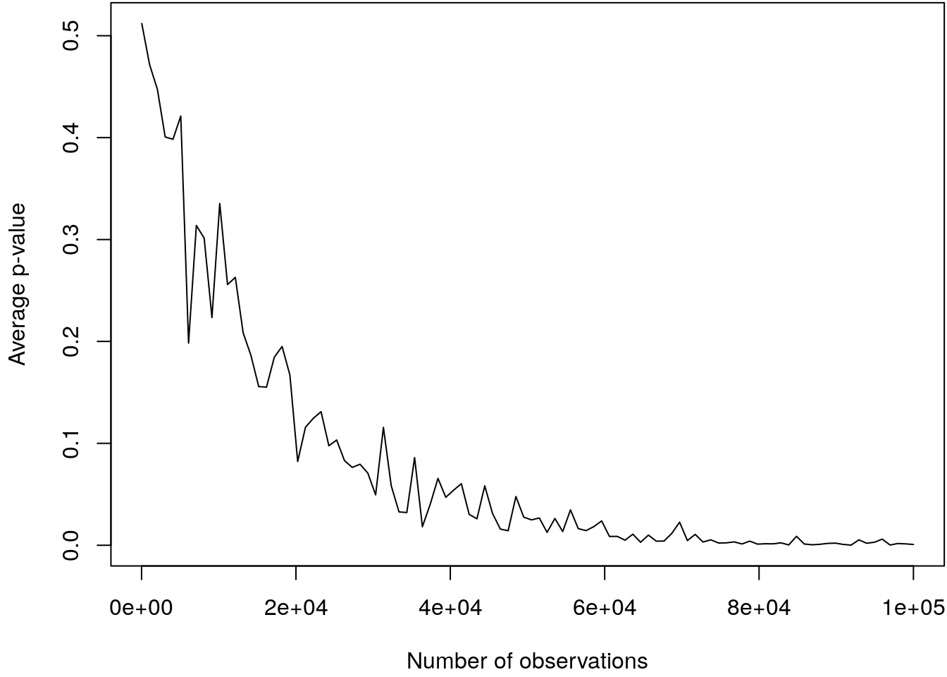

We can clearly see, that the p-values get smaller with increasing number of observations. The maximum number of observations is 1000000, which is actually not a lot. This exercise illustrates quite well that p-values using very large datasets are not very meaningful, see also the paper of Demidenko (2016).

3.2 Effect of model specification

Unfortunately, p-values are not necessarily suitable for selecting variables, since they react very sensitively to the number of observations, for example. In the chapter Model choice criteria, we have already presented better techniques for selecting variables and models. A topic we have not yet covered is the problem of correct model specification and its effect on bias, variance and prediction quality.

Effect on bias and variance

Consider the following two models: \[ \mathbf{y} = \mathbf{X} \boldsymbol{\beta}+\boldsymbol{\varepsilon} = \mathbf{X}_1 \boldsymbol{\beta}_1+ \mathbf{X}_2\boldsymbol{\beta}_2 +\boldsymbol{\varepsilon} \] and \[ \mathbf{y} = \mathbf{X}_1\boldsymbol{\beta}_1 + \mathbf{u}. \] The least squares estimators are \[ \hat{\boldsymbol{\beta}} = (\mathbf{X}^\top\mathbf{X})^{-1} \mathbf{X}^\top\mathbf{y} \quad \mbox{and} \quad \tilde{\boldsymbol{\beta}}_1 = (\mathbf{X}_1^\top\mathbf{X}_1)^{-1} \mathbf{X}_1^\top \mathbf{y} \] For the submodel, we obtain for the mean \[\begin{eqnarray*} E(\tilde{\boldsymbol{\beta}}_1)& = & E( (\mathbf{X}_1^\top\mathbf{X}_1)^{-1} \mathbf{X}_1^\top \mathbf{y}) \\ &=& (\mathbf{X}_1^\top\mathbf{X}_1)^{-1} \mathbf{X}_1^\top E( \mathbf{X}_1 \boldsymbol{\beta}_1+ \mathbf{X}_2\boldsymbol{\beta}_2 +\boldsymbol{\varepsilon} ) \\ &=& (\mathbf{X}_1^\top\mathbf{X}_1)^{-1} \mathbf{X}_1^\top (\mathbf{X}_1 \boldsymbol{\beta}_1+ \mathbf{X}_2\boldsymbol{\beta}_2) \\ &=& \boldsymbol{\beta}_1+(\mathbf{X}_1^\top\mathbf{X}_1)^{-1} \mathbf{X}_1^\top \mathbf{X}_2 \boldsymbol{\beta}_2 \end{eqnarray*}\] and for the covariance matrix \[\begin{eqnarray*} Cov(\tilde{\boldsymbol{\beta}}_1) &=& Cov((\mathbf{X}_1^\top\mathbf{X}_1)^{-1} \mathbf{X}_1^\top \mathbf{y}) = (\mathbf{X}_1^\top\mathbf{X}_1)^{-1} \mathbf{X}_1^\top \sigma^2 \mathbf{I} \mathbf{X}_1(\mathbf{X}_1^\top\mathbf{X}_1)^{-1} \\ &=& \sigma^2 (\mathbf{X}_1^\top\mathbf{X}_1)^{-1}. \end{eqnarray*}\]

So what is the effect of missing variables:

• \(\boldsymbol{\beta}_1\) is biased. An exception is the case when \(\mathbf{X}_1^\top\mathbf{X}_2 = \mathbf{0}\), i.e., every variable in \(\mathbf{X}_1\) is uncorrelated to every variable in \(\mathbf{X}_2\).
• The difference \(Cov(\hat{\boldsymbol{\beta}}) - Cov(\tilde{\boldsymbol{\beta}}_1)\) of covariance matrices is positive semi-definite. This implies that the components of the estimator \(\tilde{\boldsymbol{\beta}}_1\) based on the submodel \(\mathbf{y} = \mathbf{X}_1\boldsymbol{\beta}_1 +\mathbf{u}\) show a smaller variance than the corresponding components of the estimator \(\hat{\boldsymbol{\beta}}\) based on the correct model \(\mathbf{y}= \mathbf{X}\boldsymbol{\beta} +\boldsymbol{\varepsilon}\). Thus we have \(Var(\hat{\beta}_j) \geq Var(\tilde{\beta}_j)\).
• Moreover, situations exist where the components in \(\tilde{\boldsymbol{\beta}}_1\) based on the misspecified submodel actually show a smaller \(MSE\) than the components in \(\hat{\boldsymbol{\beta}}\), which are based on the full model, i.e., \(MSE(\hat{\beta}_j) \geq MSE(\tilde{\beta}_j)\). Hence, it is possible that a sparse model with unconsidered covariates has better statistical properties than the correctly specified full model.

And the effect of irrelevant variables:

• Even though irrelevant variables were considered, \(\hat{\boldsymbol{\beta}}\) is unbiased. Of course, the estimator \(\hat{\boldsymbol{\beta}}_1\) based on the true model is also unbiased.
• It can be shown that the estimators for the components in \(\boldsymbol{\beta}_1\) based on \(\hat{\boldsymbol{\beta}}\) have larger variance than based on \(\hat{\boldsymbol{\beta}}_1\). Thus we have \(Var(\hat{\beta}_j) \geq Var(\tilde{\beta}_j)\). If the estimated model contains irrelevant variables, then the precision of the estimators decreases.

Effect on prediction quality

For the moment, we do not assume that a model is specified correct. A model is defined by a subset \(M \subset \{0, 1, 2, \ldots ,k\}\) of included covariates. It can be shown that the expected squared prediction error is given by \[ SPSE = \sum_{i = 1}^n E(y_{n + i} - \hat{y}_{iM}) = n \sigma^2 + |M| \sigma^2 + \sum_{i=1}^n (\mu_{iM} - \mu_i)^2, \] where \(y_{n + i} = \mu_i + \varepsilon_{n + i}\), \(i = 1, \ldots, n\), and

• Irreducible error: \(n \sigma^2\).
• Variance: \(|M| \sigma^2\), becomes smaller the fewer variables are included in the model.
• Squared bias: \(\sum_{i = 1}^n (\mu_{iM} - \mu_i)^2\), becomes smaller the more variables are included in the model.

The formula of the \(SPSE\) helps to develop tools for model choice, in particular for variable selection.

Since \(\sigma^2\) and \(\mu_i\) are unknown the \(SPSE\) is not directly accessible. If indeed additional data \(y_{n + i}\) where available, we could estimate the \(SPSE\) by \[ \widehat{SPSE} = \sum_{i = 1}^n (y_{n + i} - \hat{y}_{iM}). \] However, it rarely happens that additional observations are collected. An alternative procedure is Cross validation.

Note, Cross validation only possible if the available data set is large enough, but there is no rule of thumb where to find the cutpoints. Too small data partitioning causes loss of accuracy in estimation of the regression coefficients.

However, we can try to estimate the \(SPSE\) using existing data. A naive estimator for \(SPSE\) would be the use of the squared sum of residuals \(\sum (y_i - \hat y_{iM})^2\). It can be shown that \[ E\left( \sum_{i = 1}^{n} (y_i - \hat y_{iM})^2\right) = SPSE - 2|M|\sigma^2. \] Thus a better estimate for \(SPSE\) is given by \[ \widehat{SPSE} = \sum_{i = 1}^{n} (y_i - \hat y_{iM})^2 + 2 |M|\hat{\sigma}^2. \] Keep in mind that we always use the same estimator for \(\hat{\sigma}^2\). Preferably, this estimator should be based on the full model, to keep the bias in \(\hat{\sigma}^2\) small.

This leads to the typical structure of many model choice criteria.

1. The sum of squared residuals, measures the goodness-of-fit and becomes smaller the more complex the model becomes.
2. \(2 |M| \hat \sigma^2\) measures model complexity and becomes smaller as models become simpler.

In the following we will base model and variable selection algorithms mainly on such Model choice criteria.

3.3 Selection algorithms

Thanks to the strength of modern computers, there are now a large number of algorithms, some of them computationally intensive, for variable selection and model choice. In the following we want to introduce some of the most important algorithms.

Complete model selection

Complete Model Selection (All-Subset-Selection)}: In case that the number of covariates is smaller than about 40, we can determine the best model (in the sense of a model choice criterion) with the “leaps and bounds” algorithm avoiding the computation of all models. See R package leaps (Fortran code by Alan Miller 2020).

Stepwise algorithm

This algorithm performs stepwise variable selection using an information criterion like the AIC. There are two possible step:

1. Forward Selection: Based on a starting model, forward-selection includes one additional variable in every iteration of the algorithm. The variable which offers the greatest reduction of a preselected model choice criteria (e.g., AIC) is chosen. The algorithm terminates if no further reduction is possible.
2. Backward Elimination: Starts with the full model containing all potential covariates. Subsequently, in every iteration, the covariate which provides the greatest reduction of the model choice criteria is eliminated from the model. Terminates if no further reduction is possible.

For complete stepwise selection the algorithm puts both steps together, i.e., in every iteration of the algorithm, the inclusion and the deletion of a variable are both possible. The algorithm is implemented in the step() function in R.

Exercise 3.2 Load the UsedCars data set. The data set consists of the following variables

Variable	Description
price	Sale price in 1000 Euro.
age	Age of the car in month.
kilometer	Kilometer reading in 1000 kilometer.
TIA	Month until the next TIA appointment.
abs	Does the car have abs?
sunroof	Does the car have a sunroof?

Find the best fitting regression model to predict the sale price which also accounts for nonlinearities of metric covariates age, kilometer and TIA using orthogonal polynomials of degree \(3\) and all pairwise interactions. Note, pairwise interactions can be easily set up using R’s formula syntax:

f <- y ~ x1 + x2 + x3
update(f, . ~ .^2)

## y ~ x1 + x2 + x3 + x1:x2 + x1:x3 + x2:x3

First, we need to estimate an initial model.

## Load the data.
load("data/UsedCars.rda")

## The base formula.
f <- price ~ poly(age, 3) + poly(kilometer, 3) +
  poly(TIA, 3) + abs + sunroof

## The base model.
b0 <- lm(f, data = UsedCars)

Now we define the full search scope using the formula which also includes all pairwise interactions.

## The scope we search in.
f_scope <- update(f, . ~ .^2)

The next step is to start the stepwise algorithm using the AIC for selection (which is the default).

## Run the stepwise algorithm.
b1 <- step(b0, f_scope)

## Start:  AIC=-87.69
## price ~ poly(age, 3) + poly(kilometer, 3) + poly(TIA, 3) + abs + 
##     sunroof
## 
##                                   Df Sum of Sq     RSS     AIC
## - poly(TIA, 3)                     3     1.081  90.930 -91.633
## - sunroof                          1     0.042  89.891 -89.610
## - abs                              1     0.351  90.200 -89.020
## + poly(TIA, 3):abs                 3     3.496  86.353 -88.516
## + poly(age, 3):sunroof             3     3.442  86.407 -88.409
## <none>                                          89.849 -87.691
## + poly(age, 3):abs                 3     2.715  87.134 -86.968
## + poly(age, 3):poly(TIA, 3)        9     8.521  81.328 -86.828
## + abs:sunroof                      1     0.217  89.632 -86.107
## + poly(kilometer, 3):sunroof       3     2.253  87.596 -86.058
## + poly(kilometer, 3):abs           3     1.958  87.891 -85.480
## + poly(TIA, 3):sunroof             3     0.529  89.320 -82.706
## + poly(age, 3):poly(kilometer, 3)  9     4.634  85.215 -78.798
## + poly(kilometer, 3):poly(TIA, 3)  9     4.468  85.382 -78.463
## - poly(kilometer, 3)               3    29.335 119.184 -45.094
## - poly(age, 3)                     3    77.467 167.316  13.251
## 
## Step:  AIC=-91.63
## price ~ poly(age, 3) + poly(kilometer, 3) + abs + sunroof
## 
##                                   Df Sum of Sq     RSS     AIC
## - sunroof                          1     0.045  90.975 -93.549
## - abs                              1     0.338  91.268 -92.996
## + poly(age, 3):sunroof             3     3.211  87.719 -91.817
## <none>                                          90.930 -91.633
## + poly(age, 3):abs                 3     3.109  87.821 -91.617
## + abs:sunroof                      1     0.185  90.745 -89.983
## + poly(kilometer, 3):abs           3     2.198  88.732 -89.842
## + poly(kilometer, 3):sunroof       3     2.163  88.767 -89.774
## + poly(TIA, 3)                     3     1.081  89.849 -87.691
## + poly(age, 3):poly(kilometer, 3)  9     4.627  86.303 -82.617
## - poly(kilometer, 3)               3    30.126 121.056 -48.414
## - poly(age, 3)                     3    76.804 167.734   7.681
## 
## Step:  AIC=-93.55
## price ~ poly(age, 3) + poly(kilometer, 3) + abs
## 
##                                   Df Sum of Sq     RSS     AIC
## - abs                              1     0.354  91.329 -94.881
## + poly(age, 3):abs                 3     3.144  87.831 -93.597
## <none>                                          90.975 -93.549
## + poly(kilometer, 3):abs           3     2.193  88.782 -91.745
## + sunroof                          1     0.045  90.930 -91.633
## + poly(TIA, 3)                     3     1.084  89.891 -89.610
## + poly(age, 3):poly(kilometer, 3)  9     4.666  86.309 -84.604
## - poly(kilometer, 3)               3    30.676 121.651 -49.570
## - poly(age, 3)                     3    77.123 168.098   6.053
## 
## Step:  AIC=-94.88
## price ~ poly(age, 3) + poly(kilometer, 3)
## 
##                                   Df Sum of Sq     RSS     AIC
## <none>                                          91.329 -94.881
## + abs                              1     0.354  90.975 -93.549
## + sunroof                          1     0.061  91.268 -92.996
## + poly(TIA, 3)                     3     1.064  90.265 -90.897
## + poly(age, 3):poly(kilometer, 3)  9     4.517  86.812 -85.605
## - poly(kilometer, 3)               3    30.800 122.128 -50.896
## - poly(age, 3)                     3    77.016 168.345   4.306

## Print the summary for the selected model.
summary(b1)

## 
## Call:
## lm(formula = price ~ poly(age, 3) + poly(kilometer, 3), data = UsedCars)
## 
## Residuals:
##      Min       1Q   Median       3Q      Max 
## -2.35508 -0.43535  0.01501  0.41614  3.03287 
## 
## Coefficients:
##                     Estimate Std. Error t value Pr(>|t|)    
## (Intercept)          3.39654    0.05673  59.874  < 2e-16 ***
## poly(age, 3)1       -9.24712    0.81083 -11.405  < 2e-16 ***
## poly(age, 3)2        2.44143    0.75446   3.236  0.00146 ** 
## poly(age, 3)3        0.12029    0.75110   0.160  0.87296    
## poly(kilometer, 3)1 -5.76226    0.80804  -7.131 2.97e-11 ***
## poly(kilometer, 3)2  1.84729    0.75663   2.441  0.01568 *  
## poly(kilometer, 3)3  0.20221    0.75192   0.269  0.78832    
## ---
## Signif. codes:  0 '***' 0.001 '**' 0.01 '*' 0.05 '.' 0.1 ' ' 1
## 
## Residual standard error: 0.744 on 165 degrees of freedom
## Multiple R-squared:  0.656,  Adjusted R-squared:  0.6435 
## F-statistic: 52.45 on 6 and 165 DF,  p-value: < 2.2e-16

The algorithm dropped all factor variables as well as variable TIA. The output of the algorithm needs to be read as follows. In each iteration, for each variable, the algorithm checks if adding or removing variables decreases the information criterion. The variable with most possible reduction is reported on top, e.g., in the first iteration the model term poly(TIA,3) was dropped from the model. The algorithm terminates if there is either no more change possible, or the possible reduction gets very small. The return value of function step() is an object of class "lm", i.e., all extractor and plotting functions are readily available.

## Plot estimated effects.
par(mfrow = c(1, 2), mar = c(4.1, 4.1, 0.1, 1.1))
termplot(b1, partial.resid = TRUE, se = TRUE)

Genetic algorithms

Genetic algorithms are a very interesting class of algorithms and emerged in the field of artificial intelligence. They are based on evolutionary strategies that try to mimic the process of natural selection. In this section we only discuss a particular problem that can be solved with the algorithm, namely variable selection.

1. Imagine we have a set of candidate covariates and we do not know which covariates should enter the model. For the genetic algorithm we need to index each variable (nothing new so far), but the indexing is based on \(0/1\) chromosomes, where \(0\) means the covariate is not included and \(1\) means the covariate enters the model. For example, let’s say we have a data set with 20 covariates, then the binary chromosome could be \[ \texttt{00010111001110101000}. \] Here, the first digit represents the first covariate, e.g., \(x_1\), the second digit \(x_2\), etc. Hence with the binary chromosome we can specify which covariates enter the model.
2. The second step in any genetic algorithm is initialization, meaning the algorithm randomly creates a whole population of models represented as binary chromosomes.
3. Each chromosome/model/individual is equipped with a specific fitness. The fitness function is usually the objective function that we want to optimize. In terms of model selection, the fitness function could for example be the Bayesian information criterion (BIC).
4. Having ranked the individual models the genetic algorithm now selects two parents to pass the genes to the next population. Only the fittest will be selected in this step, i.e., individuals with high fitness are more likely to be selected.
5. To create a new child, some genes of one parent and some of the other are passed on to the new child. This is done by selecting a crossover point, e.g., in the middle of the binary chromosome. Afterwards offspring are created by simply exchanging the digits, e.g., right of the crossover point. This is illustrated in the following \[ \begin{array}{c} \texttt{001001|1000} \\[-1ex] \texttt{101100|1101} \end{array} \Rightarrow \begin{array}{c} \texttt{001001|1101} \\[-1ex] \texttt{101100|1000} \end{array} \] The crossover point is marked by the vertical line. The digits right to the crossover point are exchanged. Crossover only takes place with a certain probability (crossover rate), the position of the crossover is random. The two new children are then added to the population.
6. There is also a mutation step, which randomly exchanges digits of the chromosomes according to a pre-specified rate. This step of the algorithm maintains diversity of the population and prevents the algorithm to stop in sub-optimal regions.
7. The population size is usually fixed, therefore, only the fittest remain in the newly generated population and weak individuals/models are dropped. This recombination cycle (steps 3-6) is repeated until the new population is not significantly different (in terms of the fitness function) from the previous.

Genetic algorithms avoid local maxima and will find the global optimum in complex problems more easily compared to other algorithms. Theoretical results exist that prove convergence of the algorithm, however, true genetic algorithms convergence rates are rather slow. Memetic algorithms (hybrid genetic algorithms) also include local optimization strategies which lead to faster convergence and keep advantages of genetic algorithms.

Fortunately, there is an excellent implementation of the genetic algorithm in the R package GA (Scrucca 2013, 2017, 2019). To illustrate the GA implementation we examine once more the UsedCars data set (see the exercise in section Stepwise algorithm for a description). To estimate the model we need to specify a fitness function, let’s say we use the BIC. The fitness function in hour case has one argument, which is the binary string that is passed within the main model fitting function ga() of the GA package. Using the UsedCars data, we start with a model formula that defines the full scope we want to search, i.e., we include polynomials for metric covariates and also all pairwise interactions. This can be done, e.g., by setting

## First, load the data.
load("data/UsedCars.rda")

## The base formula.
f <- price ~ poly(age, 3) + poly(kilometer, 3) +
  poly(TIA, 3) + abs + sunroof

## Now, create a big formula with all pairwise interactions.
f <- update(f, . ~ .^2)
print(f)

## price ~ poly(age, 3) + poly(kilometer, 3) + poly(TIA, 3) + abs + 
##     sunroof + poly(age, 3):poly(kilometer, 3) + poly(age, 3):poly(TIA, 
##     3) + poly(age, 3):abs + poly(age, 3):sunroof + poly(kilometer, 
##     3):poly(TIA, 3) + poly(kilometer, 3):abs + poly(kilometer, 
##     3):sunroof + poly(TIA, 3):abs + poly(TIA, 3):sunroof + abs:sunroof

The ^2 leads within function update() results the pairwise interactions. Now, each model term in the large model formula is a gene, and each gene can be activated with 1 or dropped with 0. Hence the fitness function expects a chromosome which specifies which model terms in the formula should be used for modeling. The fitness function then uses function lm() using the transformed model formula and outputs the (negative) BIC as fitness criterion.

## Function to create a new formula based on the
## original large formula f from above.
make_formula <- function(formula, which) {
  tl <- attr(terms(formula), "term.labels")
  if(length(which)) {
    tl <- tl[which]
    tl <- paste(tl, collapse = "+")
    f <- as.formula(paste("price", tl , sep = "~"))
  } else {
    f <- price ~ 1
  }
  return(f)
}

## The final fitness function. The function
## gets a binary string, creates a new formula,
## estimates a linear model and returns the
## negative BIC, since ga() searches for the
## maximum.
fitness <- function(string) {
  i <- which(string == 1)
  f <- make_formula(f, i)
  b <- lm(f, data = UsedCars)
  return(-1 * BIC(b))
}

The last step before we can start the genetic algorithm is to specify the number of model terms, i.e., the number of bits the string within the fitness function has.

nterms <- length(attr(terms(f), "term.labels"))
print(nterms)

## [1] 15

So, in total we specified \(15\) model terms and we are searching the set of terms that optimizes the BIC. The model can now be estimated with

## Load the package.
library("GA")

## Set the seed.
set.seed(123)

## Start the GA.
b <- ga("binary", fitness = fitness, nBits = nterms)

Afterwards we can extract the final binary string, create the final formula, re-estimate the model and plot the effects.

## Extract the solution.
i <- which(b@solution == 1)

## Create the final formula
f <- make_formula(f, i)
print(f)

## price ~ poly(age, 3) + poly(kilometer, 3)
## <environment: 0x563a495b7918>

## Re-estimate the model.
b <- lm(f, data = UsedCars)

## Plot effects.
par(mfrow = c(1, 2), mar = c(4.1, 4.1, 0.1, 1.1))
termplot(b, partial.resid = TRUE, se = TRUE)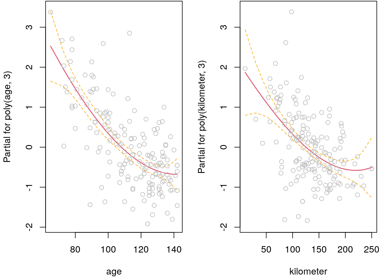

The algorithm selected only two model terms, the result is the same as in the last example exercise of section Stepwise algorithm.

Shrinkage methods

Shrinkage methods are a particularly important class of regularization techniques in statistical models. The methods presented here can be used not only to select variables, but also to estimate certain problems in the first place, and secondly to estimate sometimes highly nonlinear functions from the data, a topic we discuss in section Semiparametric regression.

Ridge regression

Ridge regression belongs to a class of penalty approaches in regression models, which aim to be a tool for variable selection. In mathematics ridge regression is known as Tikhonov regularization (https://en.wikipedia.org/wiki/Tikhonov_regularization), which has the following properties:

• General method for dealing with ill-conditioned systems.
• Regression, ill-conditioned means multicollinearity.
• Shrinkage of regression coefficients towards zero by imposing a penalty on the regression coefficients.

In ridge regression a penalty is imposed on the regression coefficients \(\boldsymbol{\beta}\), which is given by the sum of the squared coefficients \[ \text{pen}(\boldsymbol{\beta}) = \sum_{j = 1}^k\beta_j^2 = \boldsymbol{\beta}^\top\boldsymbol{\beta}. \] The penalized least squares estimator is then given by \[ \text{PLS}(\boldsymbol{\beta}) = (\mathbf{y} - \mathbf{X}\boldsymbol{\beta})^\top(\mathbf{y} - \mathbf{X}\boldsymbol{\beta}) + \lambda\boldsymbol{\beta}^\top\boldsymbol{\beta}. \] To obtain the estimator \(\hat{\boldsymbol{\beta}}\) we need to take derivatives and get \[\begin{eqnarray*} \frac{\partial}{\partial\boldsymbol{\beta}}\text{PLS}(\boldsymbol{\beta}) &=& \frac{\partial}{\partial\boldsymbol{\beta}}\left(\mathbf{y}^\top\mathbf{y} - 2\mathbf{y}^\top\mathbf{X}\boldsymbol{\beta} + \boldsymbol{\beta}^\top\mathbf{X}^\top\mathbf{X} \boldsymbol{\beta} + \lambda\boldsymbol{\beta}^\top\boldsymbol{\beta}\right) \\ &=& -2\mathbf{X}^\top \mathbf{y} + 2\mathbf{X}^\top \mathbf{X}\boldsymbol{\beta} + 2\lambda\boldsymbol{\beta}. \end{eqnarray*}\] Setting to zero and solving for \(\boldsymbol{\beta}\) yields the ridge regularized penalized least squares estimator \[ \hat{\boldsymbol{\beta}}_{\text{PLS}} = (\mathbf{X}^\top\mathbf{X} + \lambda\mathbf{I}_p)^{-1}\mathbf{X}^\top\mathbf{y}, \] where the penalization is controlled by \(\lambda \ge 0\).

The addition of \(\lambda \mathbf{I}\) to \(\mathbf{X}^\top\mathbf{X}\) leads to a regularized and invertible matrix, even if \(\mathbf{X}^\top\mathbf{X}\) is near singular due to severe collinearity. Thus, the ridge estimator often has a smaller \(MSE\) when compared to the least squares estimator.

To avoid penalization of the intercept \(\beta_0\), define the square penalty matrix \[ \mathbf{K} = \text{diag}(0, 1, \dots, 1) = \text{blockdiag}(0, \mathbf{I}_k). \] The ridge estimator is then given by \[ \hat{\boldsymbol{\beta}}_{\text{PLS}} = (\mathbf{X}^\top\mathbf{X} + \lambda\mathbf{K})^{-1}\mathbf{X}^\top\mathbf{y}. \]

The penalized least squares estimator is biased since \[ E(\hat{\boldsymbol{\beta}}_{\text{PLS}}) = E((\mathbf{X}^\top\mathbf{X} + \lambda\mathbf{K})^{-1}\mathbf{X}^\top\mathbf{y}) = (\mathbf{X}^\top\mathbf{X} + \lambda\mathbf{K})^{-1}\mathbf{X}^\top\mathbf{X}\boldsymbol{\beta}, \] as the matrices \((\mathbf{X}^\top\mathbf{X} + \lambda\mathbf{K})^{-1}\) and \(\mathbf{X}^\top\mathbf{X}\) do not cancel, unless \(\lambda = 0\). However, the shrinkage parameter needs to be selected somewhow, this can be done using Cross validation or by information criteria like the Akaike information criterion (AIC) or the Bayesian information criterion (BIC). For the second method, however, one needs an approximation of the degrees of freedom, because this is the basis for penalization. One possibility is simply to consider all non-zero coefficients for a given \(\lambda\) as momentary degrees of freedom, this is also called the “active set”. Another approximation of the degrees of freedom is to use the trace of the hat-matrix, see section Penalized regression for more details.

Fortunately, one can show that \[ \text{Var}(\hat{\beta}_{j, \text{PLS}}) < \text{Var}(\hat{\beta}_{j, \text{LS}}), \quad j = 1, \ldots, k. \]

Note that using ridge penalization (but also other shrinkage methods) it is very important to scale the data prior estimation. The reason is that the penalty is not fair if covariates live on completely different scalings and therefore the algorithm will not approach the optimum solution. In R the simplest way to scale the covariates is subtracting the mean and divide by the standard deviation as implemented in function scale(). Most implementations for shrinkage methods do scaling per default, however, if using such software make sure to read the manual properly before estimating a model.

Summary:

• When combining bias and covariance to the mean squared error one hopes to achieve a smaller MSE when choosing an appropriate smoothing parameter \(\lambda\).
• The smoothing parameter is typically determined using \(r\)-fold cross validation.
• Note, the scaling of covariates is important when applying a regularization approach. The penalty formed of squared regression coefficients assumes that all coefficients can be compared in their absolute value.

R package glmnet

Ridge regression is implemented in the R package glmnet (Friedman, Hastie, and Tibshirani 2010; N. Simon et al. 2011; Friedman et al. 2019). The main model fitting function is glmnet() and the most important arguments are:

glmnet(x, y, family = "gaussian", weights, offset = NULL,
  alpha = 1, nlambda = 100, standardize = TRUE, ...)

The model fitting function is a bit different compared to, e.g., function lm(), since it expects the user to pass the final model matrix x and the response y directly, instead of passing a model formula. The rest of the setup is pretty much similar to function lm() or glm() (just note that families are specified as character instead of family objects in function glm()).

The function computes parameter estimates \(\hat{\boldsymbol{\beta}}_{\lambda}\) using nlambda different values for the shrinkage parameter \(\lambda\). Note that the default alpha = 1 uses the LASSO penalty (see next section), for ridge regression we need to set alpha = 0. Hence, we obtain complete coefficient paths for \(\hat{\boldsymbol{\beta}}_{\lambda}\), one estimate for each \(\lambda_p,\,\, p = 1, \ldots, P\). The interesting part now is which \(\lambda_p\) to use? As mentioned above there are in principle two ways, but for the moment we try to keep things simple and use the following implementation of the BIC() method for selecting the optimum shrinkage parameter \(\lambda_p\).

BIC.glmnet <- function(object, ...) {
  call <- object$call
  dn <- as.list(call[-1])
  X <- get(as.character(dn$x))
  Y <- get(as.character(dn$y))
  n <- length(Y)
  beta <- coef(object)
  if(any(grepl("Intercept", rownames(beta))))
    X <- cbind(1, X)
  fit <- apply(beta, 2, function(b) { drop(X %*% b) })
  e <- Y - fit
  ll <- 0.5 * ( - n * (log(2 * pi) + 1 - log(n) + log(colSums(e^2))))
  bic <- -2 * ll + log(n) * object$df
  rval <- data.frame(
    "BIC" = bic,
    "lambda" = object$lambda,
    "df" = object$df
  )
  return(rval)
}

We are not going into details here, the code is mainly a simple adaption from the BIC() method for linear models and uses the “active set” (number of nonzero entries in \(\boldsymbol{\beta}\)) as approximation of the degrees of freedom. Now, after having fitted a model with glmnet() we can call the new BIC() method and just select the \(\lambda\) with the lowest BIC. This is illustrated in the following example using the MunichRent data. Recall the exercise from section Polynomial regression where we tried to find the optimum degree \(l\) of the polynomial. We can now use ridge regression to obtain a smooth penalized fit instead of increasing the degree \(l\). Therefore we set up the design matrix \(\mathbf{X}\) using orthogonal polynomials with a large degree, let’s say \(20\) and estimate the optimum shrinkage parameter using the BIC.

library("glmnet")

## Load the data.
load("data/MunichRent.rda")

## Create large design matrix.
X <- poly(MunichRent$area, 20)

## The reponse.
y <- MunichRent$rentsqm

## Estimate model using ridge penalization
## using 100 different lambdas.
b <- glmnet(X, y, nlambda = 100)

## Extract the BIC and plot.
bic <- BIC(b)
print(head(bic))

##         BIC    lambda df
## s0 14233.52 0.8298892  0
## s1 14180.20 0.7561642  1
## s2 14128.31 0.6889886  1
## s3 14084.56 0.6277808  1
## s4 14047.76 0.5720105  1
## s5 14016.88 0.5211946  1

par(mar = c(4.1 , 4.1, 0.1, 0.1))
plot(BIC ~ lambda, data = bic, type = "l")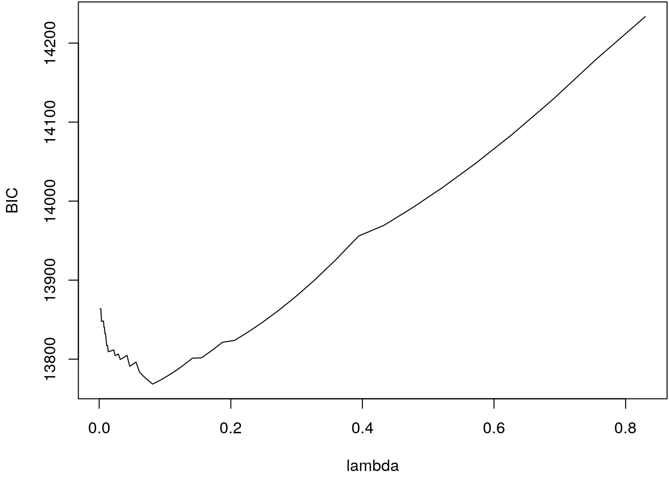

The BIC curve shows a clear minimum at

i <- which.min(bic$BIC)
print(bic$lambda[i])

## [1] 0.081081

print(bic$df[i])

## [1] 4

Now, let’ have a look at the fitted curve.

## Predict for optimum lambda iteration.
p <- predict(b, newx = X, s = bic$lambda[i])

## Plot estimated function.
par(mar = c(4.1, 4.1, 0.1, 0.1))
i <- order(MunichRent$area)
plot(rentsqm ~ area, data = MunichRent, col = rgb(0.1, 0.1, 0.1, alpha = 0.5), cex = 0.5)
lines(p[i] ~ MunichRent$area[i], lwd = 2, col = 2)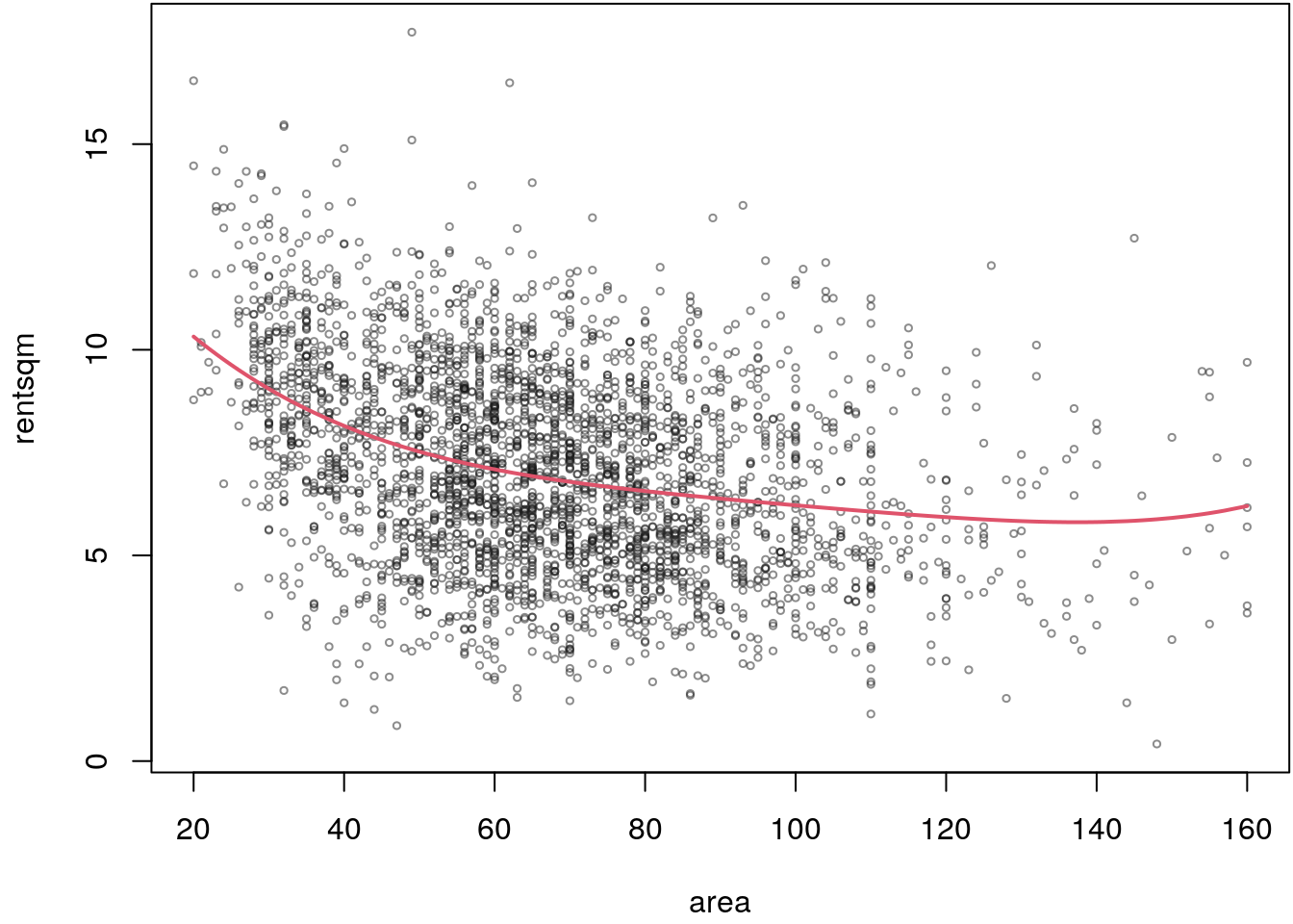

The estimated effect looks really smooth although we initially used a polynomial of degree \(20\), the ridge penalization seems to work well. The final estimate only used \(4\) degrees of freedom, i.e., all lot of columns of the design matrix are not selected by the algorithm. The user can also look at the coefficient paths which can be extracted with the coef() method (there is also a plot method, but for illustration it is good to show how the paths can be extracted “by hand”).

cb <- coef(b)
par(mar = c(4.1, 4.5, 0.1, 0.1))
matplot(bic$lambda, t(cb), type = "l", lty = 1,
  xlab = expression(lambda), ylab = expression(beta[j]))
abline(v = bic$lambda[which.min(bic$BIC)], lty = 2)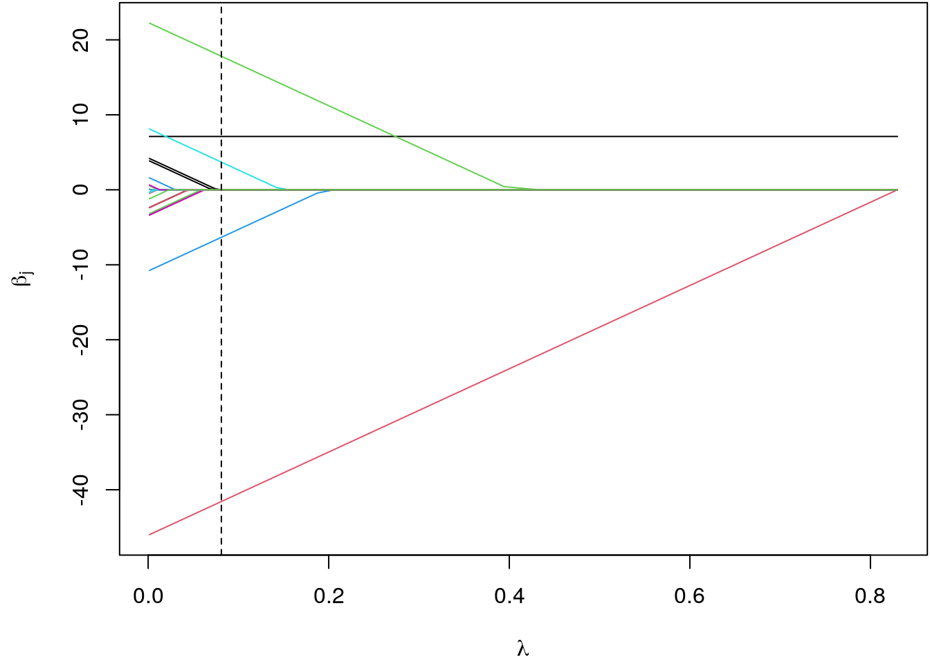

The position of the optimum shrinkage parameter is highlighted by the dashed vertical line. Here we can clearly see that only \(4\) coefficients are different from zero, all other coefficients are shrinked out of the model.

As mentioned above, another nice property of ridge regression is that we can still estimate models although the covariates are highly multi-collinear. This is illustrated in the following simulated example.

## Set the seed.
set.seed(111)

## Simulate collinear data x1 and x2.
n <- 100
x1 <- rnorm(n)
x2 <- rnorm(n, mean = x1, sd = 0.001)

## Simulate response data
y <- 3 + x1 + x2 + rnorm(n, sd = 1.2)

## First, estimate a simple linear model.
b <- lm(y ~ x1 + x2)
summary(b)

## 
## Call:
## lm(formula = y ~ x1 + x2)
## 
## Residuals:
##      Min       1Q   Median       3Q      Max 
## -2.92405 -0.84825 -0.03885  0.70018  3.03965 
## 
## Coefficients:
##             Estimate Std. Error t value Pr(>|t|)    
## (Intercept)   3.1633     0.1109  28.536   <2e-16 ***
## x1          -32.5972   109.4651  -0.298    0.767    
## x2           34.5276   109.4710   0.315    0.753    
## ---
## Signif. codes:  0 '***' 0.001 '**' 0.01 '*' 0.05 '.' 0.1 ' ' 1
## 
## Residual standard error: 1.108 on 97 degrees of freedom
## Multiple R-squared:   0.78,  Adjusted R-squared:  0.7754 
## F-statistic: 171.9 on 2 and 97 DF,  p-value: < 2.2e-16

## Now using ridge regression.
## Create design matrix for glmnet().
X <- cbind(x1, x2)

## Estimate model.
b <- glmnet(X, y, alpha = 0, lambda.min = 1e-10)

## Extract the BIC.
bic <- BIC(b)

## Extract coefficients according optimum lambda.
coef(b, s = bic$lambda[which.min(bic$BIC)])

## 3 x 1 sparse Matrix of class "dgCMatrix"
##                     1
## (Intercept) 3.1626117
## x1          0.9684079
## x2          0.9499098

The example nicely shows that the true values for \(\boldsymbol{\beta}\) could be recovered from the data quite well. The simple linear regression leads to a complete different estimate of the regression coefficients, the parameter for x1 is even negative.

LASSO

The least absolute shrinkage and selection operator (LASSO) is another penalization approach. Ridge regression does not yield a sparse solution: all estimated regression coefficients will still be slightly different from zero (however, by defining a small threshold we could still select variables).

It would be desirable not only to shrink small coefficients towards zero but to have the possibility to set some effects exactly to zero. This can be obtained by replacing the penalty of squared regression coefficients with the penalty of absolute values yielding \[ \text{pen}(\boldsymbol{\beta}) = \sum_{j = 1}^k|\beta_j| \] and \[ \hat{\boldsymbol{\beta}}_{\text{LASSO}} = \text{argmin}_{\boldsymbol{\beta}} \,\, (\mathbf{y} - \mathbf{X}\boldsymbol{\beta})^\top(\mathbf{y} - \mathbf{X}\boldsymbol{\beta}) + \lambda \sum_{j=1}^k|\beta_j|, \] which allows for true variable selection.

In contrast to ridge regression, no closed form solution for the LASSO-regularized estimate is available because the loss function is not differentiable. However, similar to the normal equations in the classical linear model we can derive \[ 2\mathbf{X}^\top\mathbf{X}\boldsymbol{\beta} + 2\mathbf{X}^\top\mathbf{y} + \lambda\sum_{j = 1}^k \text{sign}(\beta_j) = \mathbf{0}, \] which can be solved using proximal gradient methods or least-angle regression (LARS).

Using the glmnet() model fitting function LASSO-type penalization is enforced by setting alpha = 1.

Elastic net

There are some limitations of the LASSO penalty. For example, in a \(p >> n\) problem, the LASSO will select at most \(n\) covariates. In addition, if there is high multicollinearity in the data, then the LASSO will select only one variable out of the group of linearly dependent variables. To overcome these limitations Zou and Hastie (2005) proposed to combine the ridge and the LASSO in order to get the best of both worlds, this is also called elastic net regularization.

The elastic net objective is then given by \[ \hat{\boldsymbol{\beta}}_{\text{LASSO}} = \text{argmin}_{\boldsymbol{\beta}} \,\, (\mathbf{y} - \mathbf{X}\boldsymbol{\beta})^\top(\mathbf{y} - \mathbf{X}\boldsymbol{\beta}) + \lambda_1 \sum_{j=1}^k\beta_j^2 + \lambda_2 \sum_{j=1}^k|\beta_j|, \] i.e., the problem uses two shrinkage parameters \(\lambda_1\) and \(\lambda_2\). The penalty can be further simplified by \[ \text{pen}_{\text{enet}}(\boldsymbol{\beta}) = \alpha \sum_{j = 1}^k\beta_j^2 + (1 - \alpha) \sum_{j=1}^k|\beta_j| \] with \[ \alpha = \frac{\lambda_2}{\lambda_2 + \lambda_1}. \]

In function glmnet() argument alpha sets the elastic net penalty, which needs to be optimized additionally.

Exercise 3.3 In the UsedCars example it is unclear which covariates and interactions should enter the model. Estimate a model which considers all possible interactions and models all metric covariates as polynomials of degree \(10\). Apply variable selection using the elastic net penalty as implemented in function glmnet(). The optimum penalty should be selected using the BIC (see the implementation above).

For finding the optimum \(\alpha\) parameter within the elastic net, we use a simple grid search. Before doing so, we need to create the design matrix \(\mathbf{X}\). This can be done using a model formula and the model.matrix() function.

load("data/UsedCars.rda")

## For creating the design matrix for glmnet()
## we need a formula which can be send to the
## model.matrix() function. The base formula is:
f <- price ~ poly(age, 10) + poly(kilometer, 10) +
  poly(TIA, 10) + abs + sunroof - 1

## Note, we need to drop the intercept, which is
## included in glmnet() later.

## The formula including all pairwise intercation.
f <- update(f, . ~ .^2)
print(f)

## price ~ poly(age, 10) + poly(kilometer, 10) + poly(TIA, 10) + 
##     abs + sunroof + poly(age, 10):poly(kilometer, 10) + poly(age, 
##     10):poly(TIA, 10) + poly(age, 10):abs + poly(age, 10):sunroof + 
##     poly(kilometer, 10):poly(TIA, 10) + poly(kilometer, 10):abs + 
##     poly(kilometer, 10):sunroof + poly(TIA, 10):abs + poly(TIA, 
##     10):sunroof + abs:sunroof - 1

## Create the design matrix.
X <- model.matrix(f, data = UsedCars)
print(dim(X))

## [1] 172 394

## The response.
y <- UsedCars$price

## Estimate models using a grid search for the
## alpha parameter.
n <- 100
alpha <- seq(0, 1, length = n)
bic <- rep(NA, n)
for(i in 1:n) {
  b <- glmnet(X, y, nlambda = 100, alpha = alpha[i])
  bic[i] <- min(BIC(b)$BIC)
}

## Plot the BIC curve.
par(mar = c(4.1, 4.1, 0.5, 0.1))
plot(bic ~ alpha, type = "l",
 xlab = expression(alpha), ylab = "BIC")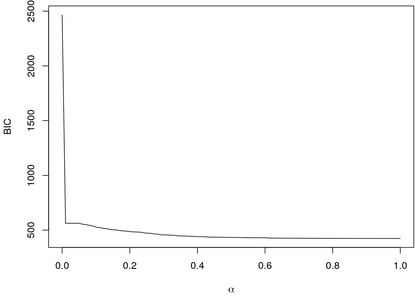

## Optimum alpha.
print(alpha[i <- which.min(bic)])

## [1] 1

In this case the grid search results in \(\alpha = 1\). Now we re-estimate the model and extract the optimum parameters again using the BIC.

b <- glmnet(X, y, nlambda = 100, alpha = alpha[i])

## Extract BIC.
bic <- BIC(b)

## Show the BIC curve.
par(mar = c(4.1 , 4.1, 0.1, 0.1))
plot(BIC ~ lambda, data = bic, type = "l")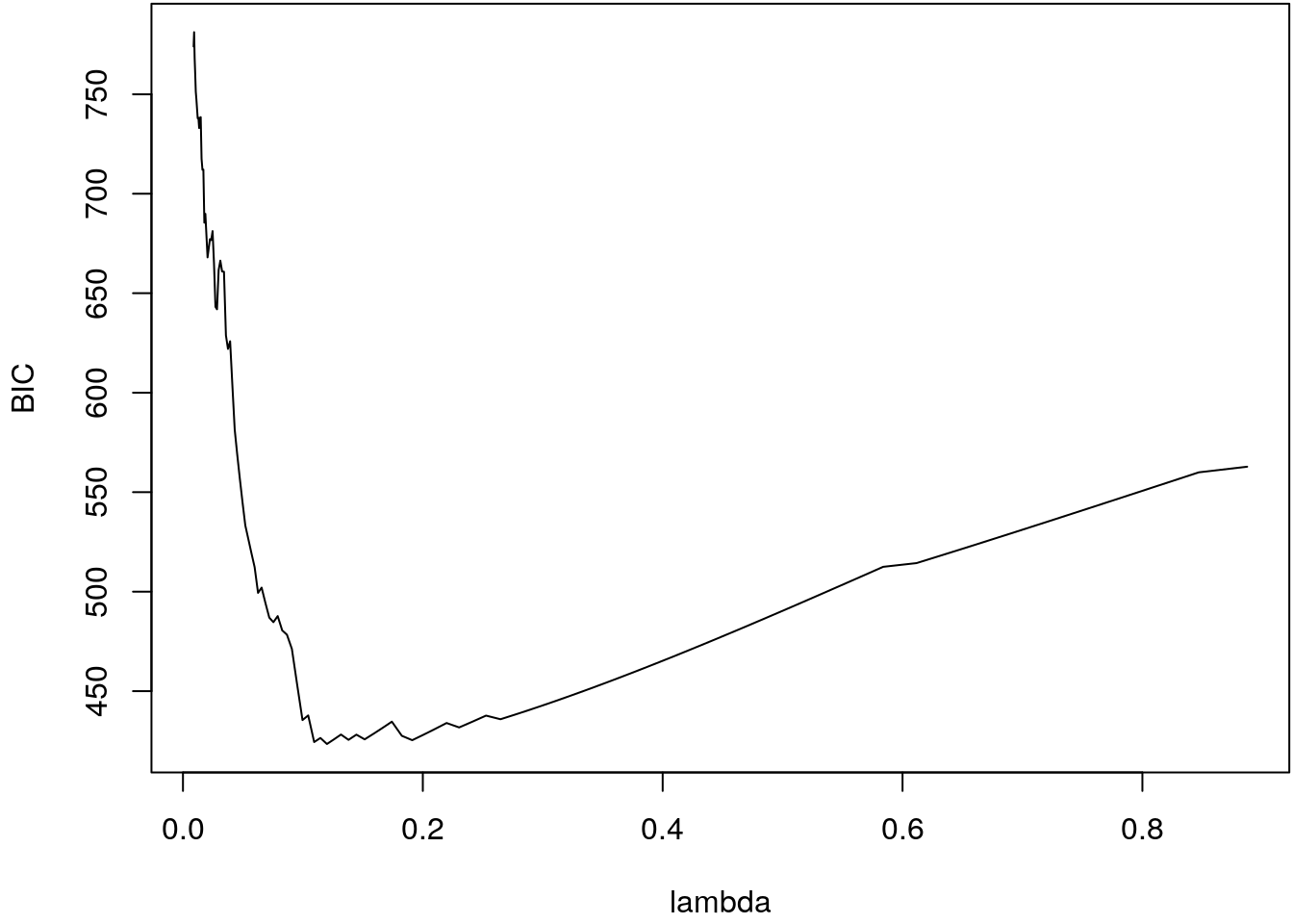

## Extract parameters at minimum BIC.
cb <- coef(b)
cb <- cb[, which.min(bic$BIC)]

## Only show non-zero coefficients.
print(cb[abs(cb) > 0])

##                         (Intercept)                      poly(age, 10)1 
##                           3.3498196                          -7.9315820 
##                      poly(age, 10)2                poly(kilometer, 10)1 
##                           0.3781845                          -4.5122607 
## poly(age, 10)1:poly(kilometer, 10)1       poly(age, 10)7:poly(TIA, 10)2 
##                          13.8079707                          -1.8892463 
##       poly(age, 10)6:poly(TIA, 10)4       poly(age, 10)7:poly(TIA, 10)4 
##                         -13.0551085                           4.7010924 
##       poly(age, 10)7:poly(TIA, 10)6       poly(age, 10)3:poly(TIA, 10)9 
##                         -10.7842704                           3.9549927

## Plot coefficient paths.
cb <- coef(b)
par(mar = c(4.1, 4.5, 0.1, 0.1))
matplot(bic$lambda, t(cb), type = "l", lty = 1,
  xlab = expression(lambda), ylab = expression(beta[j]))
abline(v = bic$lambda[which.min(bic$BIC)], lty = 2)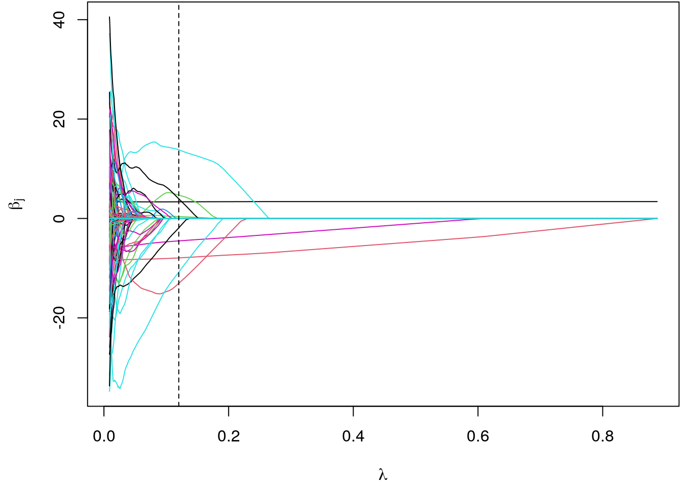

The elastic net in combination with the BIC selected \(3\) covariates to be included in the model. In comparison to the example presented in section Stepwise algorithm and Genetic algorithms, the shrinkage method also selected interaction effects.

Boosting

In boosting regularization is implicitly achieved through early stopping of an iterative stepwise algorithm. Boosting is a general and versatile regularization approach since estimation problems are described in terms of a loss function and, as a consequence, boosting can also be applied beyond the linear model, e.g., in robust regression or generalized linear models for non-Gaussian responses.

Consider the linear model \[\begin{eqnarray*} y_i &=& \eta_i + \varepsilon_i = \mathbf{x}_i^\top\boldsymbol{\beta} + \varepsilon_i, \quad i = 1, \ldots, n, \end{eqnarray*}\] with the standard predictor \(\eta_i = \mathbf{x}_i^\top\boldsymbol{\beta}\). We are interested in situations where the ordinary least squares estimate is not optimal, e.g., the number of regression coefficients is large, the design matrix is close to collinear, or we need to find suitable subset of covariates.

The basic boosting algorithm is described by the following:

1. Choose an initial estimate \(\hat{\boldsymbol{\beta}}^{(0)}\) and set \(t = 1\).
2. Compute the current residuals \(\mathbf{u} = \mathbf{y} - \mathbf{X}\hat{\boldsymbol{\beta}}^{(t-1)}\) and the corresponding least squares estimate \(\hat{\mathbf{b}} = (\mathbf{X}^\top\mathbf{X})^{-1}\mathbf{X}^\top\mathbf{u}\). Perform the update \[ \hat{\boldsymbol{\beta}}^{(t)} = \hat{\boldsymbol{\beta}}^{(t-1)} + \nu\hat{\mathbf{b}} \] with \(0 < \nu < 1\) and set \(t = t + 1\).
3. Iterate step 2 for a fixed number of iterations \(m_{\text{stop}}\).

The factor \(\nu\) implicitly implements regularization since \(-\) when stopping early enough \(-\) the multiplication with \(\nu\) yields a proportional shrinkage of the estimates analogous to ridge regression.

Now consider \[ \left. \frac{\partial}{\partial\boldsymbol{\beta}} LS(\boldsymbol{\beta}) \right|_{\boldsymbol{\beta} = \hat{\boldsymbol{\beta}}^{(0)}} = -2 \mathbf{X}^\top \left( \mathbf{y} - \mathbf{X}\hat{\boldsymbol{\beta}}^{(0)} \right). \] This derivative indicates the direction towards the least squares estimate and would be zero if the initial value is already the least squares estimate since it then coincides with the normal equations.

To achieve regularization, we only do small steps towards the solution so that \[ \hat{\boldsymbol{\beta}}^{(1)} = \hat{\boldsymbol{\beta}}^{(0)} + \nu \hat{\mathbf{b}} \] where \(\hat{\mathbf{b}} = (\mathbf{X}^\top\mathbf{X})^{-1}\mathbf{X}^\top\mathbf{u}\) is the least squares estimate obtained from the residuals \(\mathbf{u} = \mathbf{y} - \mathbf{X}\hat{\boldsymbol{\beta}}^{(0)}\).

Instead of updating the whole parameter vector \(\boldsymbol{\beta}\) in each iteration of the boosting algorithm, the problem can also be split into separate components. This is implemented as follows: First compute least squares estimates for all covariates separately, i.e. \[ \hat{b}_j = (\mathbf{x}_j^\top\mathbf{x}_j)^{-1}(\mathbf{x}_j)^\top\mathbf{u} = \frac{\displaystyle \sum_{i = 1}^n(x_{ij} - \bar{x}_j)u_i}{\displaystyle \sum_{i = 1}^n(x_{ij} - \bar{x}_j)^2}, \quad j = 0, \ldots, k, \] based on the current residuals \(\mathbf{u}\) where \(\mathbf{x}_j = (x_{1j}, \ldots, x_{nj})^\top\) is the column of \(\mathbf{X}\) corresponding to the \(j\)th covariate and \(\bar{x}_j\) is the average of the covariate values. We then do not update all coefficients, but rather only the one that leads to the largest reduction in the least squares criterion, i.e., we determine \[ j^* = \text{argmin}_{j = 0, \ldots, k} \sum_{i = 1}^n(u_i-x_{ij}\hat{b}_j)^2, \] and then update the coefficients using \[\begin{eqnarray*} \hat{\beta}_{j^*}^{(1)} &=& \hat{\beta}_{j^*}^{(0)} + \nu \hat{b}_{j^*},\\ \hat{\beta}_{j}^{(1)} &=& \hat{\beta}_{j}^{(0)}, \quad j\neq j^*. \end{eqnarray*}\]

The main challenge in gradient boosting is to finde the optimum stopping iteration, the optimum amount of shrinkage. This can be done, e.g., by cross validation or again selection using the AIC or BIC. Using information criteria is however computationally challenging, since the \(n \times n\) hat-matrix needs to be computed and updated in each iteration. For probelms with a lot of observations this is not feasible anymore.

The real great advantage of gradient boosting is that the method can be applied to any problem where we can specify a differentiable loss function. This is also called generic component wise boosting. The algorithm is only slightly different since the “residuals” are now given by the negative gradient of the general loss function.

1. Initialize the regression coefficients, e.g., as \[ \beta_0^{(0)} = \bar{y}\quad\mbox{and}\quad \beta_j^{(0)} = 0,\ j = 1, \ldots, k, \] choose a number of iterations \(m_{\text{stop}}\) and set \(t = 0\).
2. Increase \(t\) by 1. Compute the negative gradients (“residuals”) \[\begin{eqnarray*} u_i = - \frac{\partial}{\partial \eta} \rho(y_i,\eta)|_{\eta = \hat{\eta}^{(t-1)}_i},\ i = 1, \ldots , n, \end{eqnarray*}\] where \(\rho\) is a general loss function, e.g., the least squares criterion, describing the estimation problem.
3. Fit separate linear models for all covariates, i.e., obtain \[ \hat{b}_j = (\mathbf{x}_j^\top\mathbf{x}_j)^{-1}(\mathbf{x}_j)^\top\mathbf{u}, \ j = 0, \ldots, k \] and determine the best-fitting variable via \[ j^* = \text{argmin}_{j = 0, \ldots, k} \sum_{i = 1}^n(u_i - x_{ij}\hat{b}_j)^2. \]
4. Update the coefficients and the predictor: \[\begin{eqnarray*} \eta_i^{(t)} &=& \eta_i^{(t-1)} + \nu \cdot x_{ij^*}\hat{b}_{j^*}\\ \hat{\beta}_{j^*}^{(1)} &=& \hat{\beta}_{j^*}^{(0)} + \nu \hat{b}_{j^*}\\ \hat{\beta}_{j}^{(1)} &=& \hat{\beta}_{j}^{(0)}, \quad j\neq j^*. \end{eqnarray*}\]
5. Iterate steps 2–4 until \(t = m_\text{stop}\).

R package mboost

Component wise boosting is implemented in the R package mboost (Hothorn et al. 2010, 2020; Hofner et al. 2014). The main model fitting function for linear models is glmboost() and the most important arguments are:

glmboost(formula, data = list(), weights = NULL,
  offset = NULL, family = Gaussian(),
  na.action = na.pass, contrasts.arg = NULL,
  center = TRUE, ...)

Note again that covariates are centered per default. The reason is again, that similar to ridge and LASSO regression covariates should be scaled equally, otherwise the comparison that decides which covariate to update is not fair and the optimum amount of shrinkage, the best model, cannot be selected properly.

We illustrate the use of mboost using once more the UsedCars data and the exercise from the previous section. Instead of elastic net we apply component wise gradient boosting.

library("mboost")
load("data/UsedCars.rda")

## For creating the design matrix for glmnet()
## we need a formula which can be send to the
## model.matrix() function. The base formula is:
f <- price ~ poly(age, 10) + poly(kilometer, 10) +
  poly(TIA, 10) + abs + sunroof

## Note, we need to drop the intercept, which is
## included in glmnet() later.

## The formula including all pairwise intercation.
f <- update(f, . ~ .^2)
print(f)

## price ~ poly(age, 10) + poly(kilometer, 10) + poly(TIA, 10) + 
##     abs + sunroof + poly(age, 10):poly(kilometer, 10) + poly(age, 
##     10):poly(TIA, 10) + poly(age, 10):abs + poly(age, 10):sunroof + 
##     poly(kilometer, 10):poly(TIA, 10) + poly(kilometer, 10):abs + 
##     poly(kilometer, 10):sunroof + poly(TIA, 10):abs + poly(TIA, 
##     10):sunroof + abs:sunroof

## Estimate model with gradient boosting.
b <- glmboost(f, data = UsedCars, control = boost_control(mstop = 1000))

Similar to ridge and LASSO regression, we can inspect the coefficient paths.

par(mar = c(4.1, 4.1, 0.5, 15))
plot(b, main = "")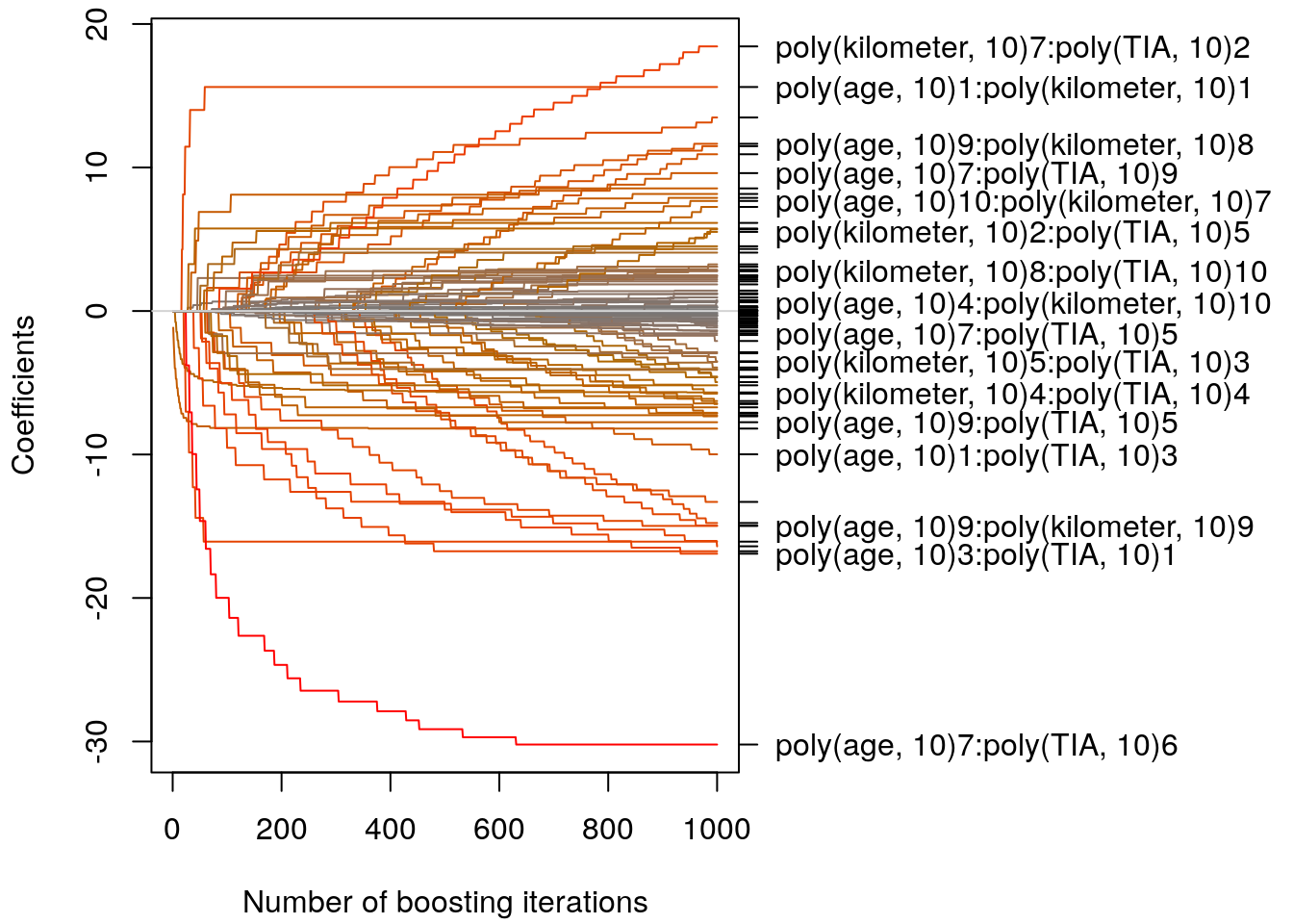

Let’s select the optimum stopping iteration using \(10\)-fold Cross validation.

cv10f <- cv(model.weights(b), type = "kfold")
cvm <- cvrisk(b, folds = cv10f, papply = lapply)
mstop(cvm)

## [1] 51

par(mar = c(4.1, 4.1, 4.1, 0.1))
plot(cvm)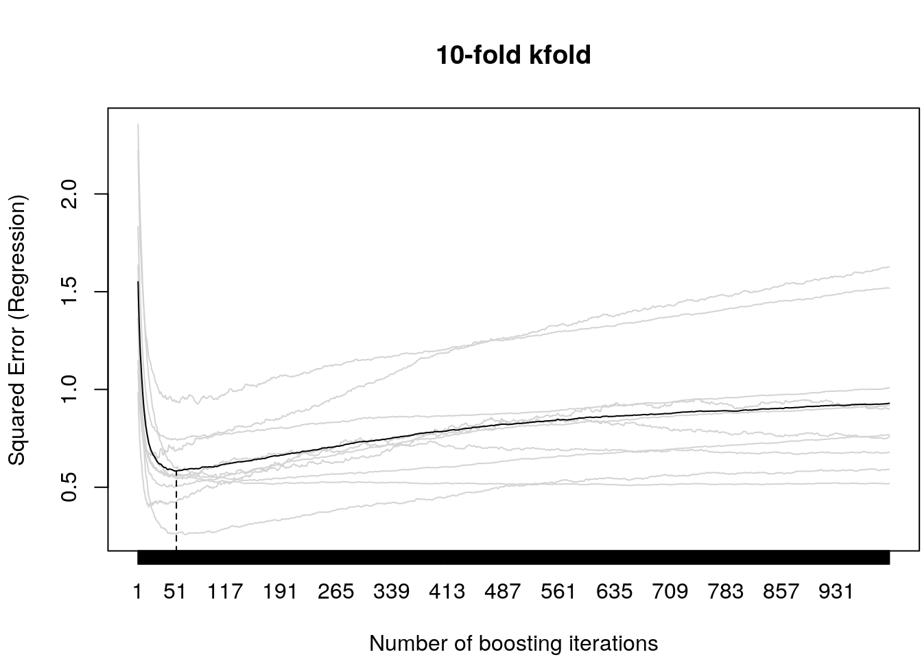

According the CV score, the optimum stopping iteration is \(51\). The estimated coeffcients can then be extracted by

m <- b[mstop(cvm)]
summary(m)

## 
##   Generalized Linear Models Fitted via Gradient Boosting
## 
## Call:
## glmboost.formula(formula = f, data = UsedCars, control = boost_control(mstop = 1000))
## 
## 
##   Squared Error (Regression) 
## 
## Loss function: (y - f)^2 
##  
## 
## Number of boosting iterations: mstop = 51 
## Step size:  0.1 
## Offset:  3.396541 
## 
## Coefficients: 
##                          (Intercept)                       poly(age, 10)1 
##                          -0.05482273                          -8.03627786 
##                       poly(age, 10)2                 poly(kilometer, 10)1 
##                           0.40836472                          -4.70946554 
##  poly(age, 10)1:poly(kilometer, 10)1 poly(age, 10)10:poly(kilometer, 10)3 
##                          14.00928719                           2.29694902 
##        poly(age, 10)7:poly(TIA, 10)2        poly(age, 10)6:poly(TIA, 10)4 
##                          -4.70272126                         -14.42037725 
##        poly(age, 10)7:poly(TIA, 10)4        poly(age, 10)7:poly(TIA, 10)6 
##                           5.74734601                         -14.63891413 
##        poly(age, 10)4:poly(TIA, 10)7        poly(age, 10)3:poly(TIA, 10)9 
##                           1.76441874                           6.90223046 
## attr(,"offset")
## [1] 3.396541
## 
## Selection frequencies:
##                       poly(age, 10)1                 poly(kilometer, 10)1 
##                           0.27450980                           0.23529412 
##        poly(age, 10)6:poly(TIA, 10)4        poly(age, 10)7:poly(TIA, 10)6 
##                           0.09803922                           0.09803922 
##  poly(age, 10)1:poly(kilometer, 10)1        poly(age, 10)3:poly(TIA, 10)9 
##                           0.07843137                           0.05882353 
##                       poly(age, 10)2        poly(age, 10)7:poly(TIA, 10)2 
##                           0.03921569                           0.03921569 
##        poly(age, 10)7:poly(TIA, 10)4 poly(age, 10)10:poly(kilometer, 10)3 
##                           0.03921569                           0.01960784 
##        poly(age, 10)4:poly(TIA, 10)7 
##                           0.01960784

Which yields very similar results as in the elastic net example from the last section.

References

Demidenko, Eugene. 2016. “The p-Value You Can’t Buy.” The American Statistician 70 (1): 33–38. https://doi.org/10.1080/00031305.2015.1069760.

Fortran code by Alan Miller, Thomas Lumley based on. 2020. Leaps: Regression Subset Selection. https://CRAN.R-project.org/package=leaps.

Friedman, Jerome, Trevor Hastie, and Robert Tibshirani. 2010. “Regularization Paths for Generalized Linear Models via Coordinate Descent.” Journal of Statistical Software 33 (1): 1–22. http://www.jstatsoft.org/v33/i01/.

Friedman, Jerome, Trevor Hastie, Rob Tibshirani, Balasubramanian Narasimhan, and Noah Simon. 2019. Glmnet: Lasso and Elastic-Net Regularized Generalized Linear Models. https://CRAN.R-project.org/package=glmnet.

Green W., H. 2017. Econometric Analysis. Pearson.

Hofner, Benjamin, Andreas Mayr, Nikolay Robinzonov, and Matthias Schmid. 2014. “Model-Based Boosting in R: A Hands-on Tutorial Using the R Package Mboost.” Computational Statistics 29: 3–35.

Hothorn, Torsten, Peter Buehlmann, Thomas Kneib, Matthias Schmid, and Benjamin Hofner. 2010. “Model-Based Boosting 2.0.” Journal of Machine Learning Research 11: 2109–13.

———. 2020. mboost: Model-Based Boosting. https://CRAN.R-project.org/package=mboost.

Scrucca, Luca. 2013. “GA: A Package for Genetic Algorithms in R.” Journal of Statistical Software 53 (4): 1–37. http://www.jstatsoft.org/v53/i04/.

———. 2017. “On Some Extensions to GA Package: Hybrid Optimisation, Parallelisation and Islands Evolution.” The R Journal 9 (1): 187–206. https://journal.r-project.org/archive/2017/RJ-2017-008.

———. 2019. GA: Genetic Algorithms. https://CRAN.R-project.org/package=GA.

Simon, Noah, Jerome Friedman, Trevor Hastie, and Rob Tibshirani. 2011. “Regularization Paths for Cox’s Proportional Hazards Model via Coordinate Descent.” Journal of Statistical Software 39 (5): 1–13. http://www.jstatsoft.org/v39/i05/.

Wooldridge, Jeffrey Marc. 2016. Introductory Econometrics: A Modern Approach. South-Western Cengage Learning.

Zou, Hui, and Trevor Hastie. 2005. “Regularization and Variable Selection via the Elastic Net.” Journal of the Royal Statistical Society, Series B 67: 301–20.