Chapter 6 Bayesian models

6.1 Introduction

Bayesian statistics is based on a few simple rules of probability. This is one of the chief advantages of the Bayesian approach.

All of the things that we would like to do, such as estimate the parameters of a model, compare different models or obtain predictions from the model, involve the same rules of probability.

Let us consider two random variables \(A\) and \(B\). The rules of probability imply \[ p(A, B) = p(A | B)p(B), \] where \(p(A, B)\) is the joint probability density function (PDF) of \(A\) and \(B\), \(p(A | B)\) is the PDF of \(A\) occurring conditional on \(B\) having occurred and \(p(B)\) is the marginal PDF of \(B\).

Alternatively, we can write \[ p(A, B) = p(B | A)p(A). \]

Equating the two expressions for \(p(A, B)\) and rearranging provides us with the Bayes’rule, which lies at the heart of Bayesian statistics \[ p(B | A) = \frac{p(A | B)p(B)}{p(A)}. \]

Lets think of the simple linear regression. In this model interest often centers on the coefficients in the regression, and the researcher is interested in estimating these coefficients.

Let \(\mathbf{y}\) be a response vector and \(\boldsymbol{\theta}\) be a vector or matrix which contains the parameters of the model which seeks to explain \(\mathbf{y}\).

Bayesian statistics uses Bayes’ rule to do so, i.e., we replace \(B\) with \(\boldsymbol{\theta}\) and \(A\) with \(\mathbf{y}\) \[ p(\boldsymbol{\theta} | \mathbf{y}) = \frac{p(\mathbf{y} | \boldsymbol{\theta}) p(\boldsymbol{\theta})}{p(\mathbf{y})} = \frac{p(\mathbf{y} | \boldsymbol{\theta}) p(\boldsymbol{\theta})}{c}. \]

Bayesians treat \(p(\boldsymbol{\theta} | \mathbf{y})\) as being of fundamental interest. That is, it directly addresses the question “Given the data, what do we know about \(\boldsymbol{\theta}\)?”.

Treating \(\boldsymbol{\theta}\) as a random variable is controversial, e.g., the frequentist econometrician says that \(\boldsymbol{\theta}\) is not a random variable.

However, Bayesian statistics is based on a subjective view of probability, which argues that our uncertainty about anything unknown can be expressed by the rules of probability.

The posterior density

So, our interest lies in \(p(\boldsymbol{\theta} | \mathbf{y})\). Insofar as we are only interested in learning about \(\boldsymbol{\theta}\) we can write \[ p(\boldsymbol{\theta} | \mathbf{y}) \propto p(\mathbf{y} | \boldsymbol{\theta}) p(\boldsymbol{\theta}). \]

The term \(p(\boldsymbol{\theta} | \mathbf{y})\) is referred to as the posterior density, the PDF for the data given the parameters of the model.

\(p(\mathbf{y} | \boldsymbol{\theta})\) is the likelihood function and \(p(\boldsymbol{\theta})\) the prior density.

You often see this relationship referred to as \[ \text{posterior} \propto \text{likelihood} \times \text{prior}. \]

The prior, \(p(\boldsymbol{\theta})\), does not depend upon the data, but can of course be determined by other findings, e.g., from data collected in another study. For example: Let \(A\) be the event that we sell ice cream and \(B\) the event of the weather. Then we could ask ourselves what is the probability of selling ice cream on a particular day, considering the nature of the weather. Here the prior \(p(A = \text{"ice cream sale"})\), i.e., the (marginal) probability of selling ice cream regardless of the type of weather outside. \(p(A)\) is known as the prior because we might already know the marginal probability of the sale of ice cream. For example, I could look at data that said \(30\) people out of a potential \(100\) actually bought ice cream at some shop somewhere. So my \(p(A = \text{"ice cream sale"}) = 30/100 = 0.3\), prior to me knowing anything about the weather.

Accordingly, it contains any information available about \(\boldsymbol{\theta}\), i.e., it summarizes what you know about \(\boldsymbol{\theta}\) prior to seeing the data, i.e., our strengths on beliefs about the parameters based on the previous experience.

In Bayesian statistics we have three types of priors, informative, non-informative and data-based priors.

Connection to regression models

The likelihood function, \(p(\mathbf{y} | \boldsymbol{\theta})\), is the density of the data conditional on the parameters of the model. It is often referred to as the data generating process.

E.g., in the linear regression model, we commonly assume that the errors are normally distributed, this implies that \(p(\mathbf{y} | \boldsymbol{\theta})\) is a normal density, which depends on \(\boldsymbol{\theta}\) (i.e., \(\boldsymbol{\beta}\), \(\sigma^2\)).

The posterior, \(p(\boldsymbol{\theta} | \mathbf{y})\), is the density which is of fundamental interest. It summarizes all we know about \(\boldsymbol{\theta}\) after (i.e., posterior to) seeing the data.

Hence, Bayes’ rule implies that the data allows us to update our prior beliefs about \(\boldsymbol{\theta}\), which results in the posterior, combining data and non-data information.

The following illustrates the influence of four different prior PDFs on the posterior density.

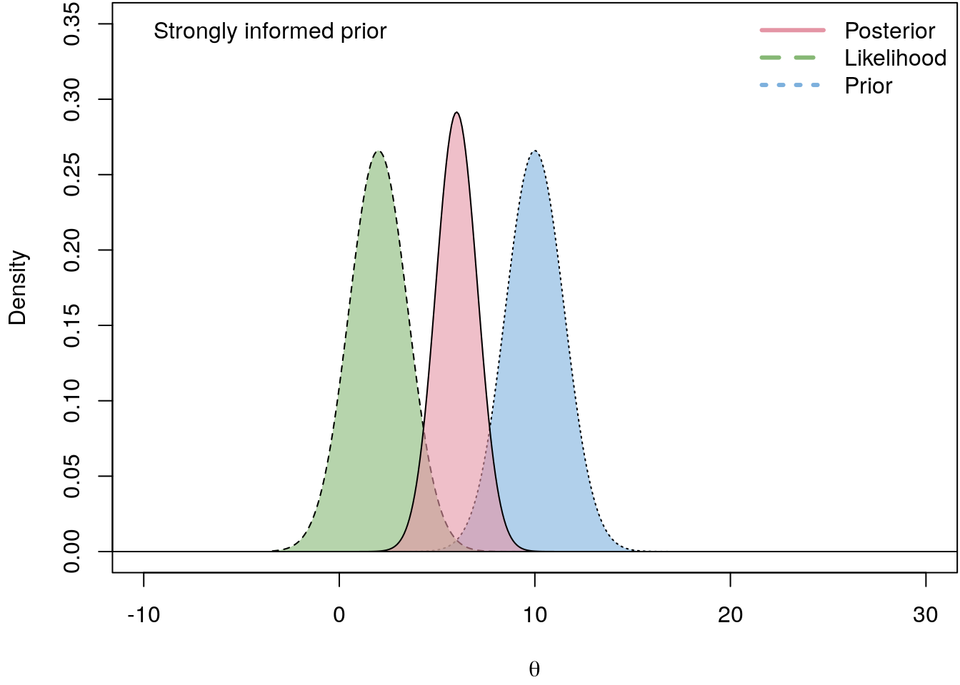
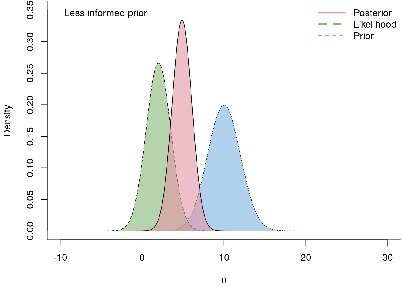
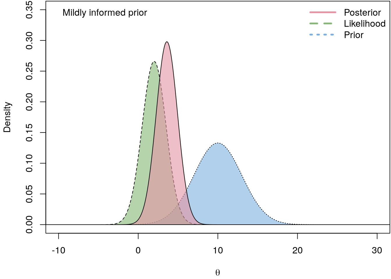
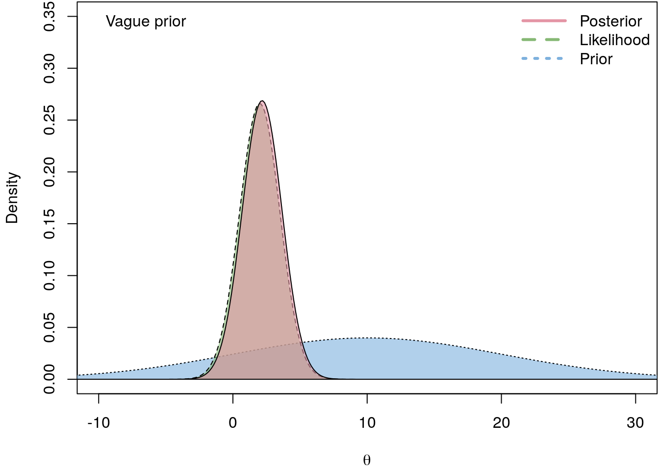
I.e., the less informative the prior the closer is the log-likelihood to the actual posterior. hence, in a regression setting we usually do not have good prior beliefs about \(\boldsymbol{\theta}\), therefore we commonly use vague priors which are almost non-informative.

Comparing models

Now suppose we have \(i = 1, \ldots, m\) models \(M_i\), and \(M_i\) depends on parameters \(\boldsymbol{\theta}_i\).

In cases where many models are being entertained, it is important to be explicit about which model is under consideration.

The posterior for the parameters calculated using \(M_i\) is \[ p(\boldsymbol{\theta}_i | \mathbf{y}, M_i) = \frac{p(\mathbf{y} | \boldsymbol{\theta}_i, M_i) p(\boldsymbol{\theta}_i | M_i)}{p(\mathbf{y} | M_i)}. \]

Once again we could use Bayes’ rule to derive a probability statement about what we do not know conditional on what we know. This means the posterior model probability can be used to assess the degree of support for \(M_i\) \[ p(M_i | \mathbf{y}) = \frac{p(\mathbf{y} | M_i)p(M_i)}{p(\mathbf{y})}. \]

\(p(M_i)\) is referred to as the . Since it does not involve the data, it measures how likely we believe \(M_i\).

\(p(\mathbf{y} | M_i)\) is called the marginal likelihood and is calculated by integrating both sides of \[ p(\boldsymbol{\theta}_i | \mathbf{y}, M_i) = \frac{p(\mathbf{y} | \boldsymbol{\theta}_i, M_i) p(\boldsymbol{\theta}_i | M_i)}{p(\mathbf{y} | M_i)}. \] with respect to \(\boldsymbol{\theta}_i\). We use the fact that \[ \int p(\boldsymbol{\theta}_i | \mathbf{y}, M_i)d\boldsymbol{\theta}_i = 1, \] and rearranging yields \[ p(\mathbf{y} | M_i) = \int p(\mathbf{y} | \boldsymbol{\theta}_i, M_i) p(\boldsymbol{\theta}_i | M_i)d\boldsymbol{\theta}_i. \]

Since \(p(\mathbf{y})\) is often hard to calculate directly, it is common to compare two models , \(i\) and \(j\), using the , which is \[ \frac{p(M_i | \mathbf{y})}{p(M_j | \mathbf{y})} = \frac{p(\mathbf{y} | M_i)p(M_i)} {p(\mathbf{y} | M_j)p(M_j)}. \]

Note that, since \(\mathbf{y}\) is common to both models, it cancels out when we take the ratio.

Sometimes we want to compare models having the same prior weights, that is \(p(M_i) = p(M_j)\), which reduces the posterior odds ratio to \[ \frac{p(\mathbf{y} | M_i)}{p(\mathbf{y} | M_j)} \] i.e., the ratio of the marginal likelihoods, which is called the Bayes factor.

Prediction

Finally, we are also interested in prediction, i.e., given the observed data \(\mathbf{y}\), we want to predict some future unobserved data \(\mathbf{y}^{\star}\).

Following Bayes, we should summarize our uncertainty about what we do not know through a conditional probability statement, the \[ p(\mathbf{y}^{\star} | \mathbf{y}). \]

We can write the predictive density in a more convenient form \[ p(\mathbf{y}^{\star} | \mathbf{y}) = \int p(\mathbf{y}^{\star}, \boldsymbol{\theta} | \mathbf{y})d \boldsymbol{\theta} \] which gives \[ p(\mathbf{y}^{\star} | \mathbf{y}) = \int p(\mathbf{y}^{\star} | \mathbf{y}, \boldsymbol{\theta}) p(\boldsymbol{\theta} | \mathbf{y})d\boldsymbol{\theta}. \]

The equation of the posterior does not involve any integrals, but presentation of information about parameters can often involve substantial computation.

It is quite difficult to present all the information about \(p(\boldsymbol{\theta} | \mathbf{y})\), only if \(\boldsymbol{\theta}\) has a simple form or \(\theta\) is one-dimensional, it is possible to do so, e.g. by graphing the posterior density.

Usually, we want a point estimate, a best guess what \(\boldsymbol{\theta}\) actually is, however, this can involve integration, which might not be evaluable analytically.

Let us suppose we want to evaluate the posterior mean as a point estimate for \(\boldsymbol{\theta} = (\theta_1, \ldots, \theta_k)^\top\). The posterior mean for any element of \(\boldsymbol{\theta}\) is \[ E(\theta_j | \mathbf{y}) = \int \theta_j p(\boldsymbol{\theta} | \mathbf{y})d\boldsymbol{\theta}. \]

In addition to a point estimate, it is usually desirable to present a measure of the degree of uncertainty associated with the point estimate, the posterior standard deviation \[ Var(\theta_j | \mathbf{y}) = E(\theta_j^2 | \mathbf{y}) - \left(E(\theta_j | \mathbf{y})\right)^2 \] which requires evaluation of the posterior mean as well as \[ E(\theta_j^2 | \mathbf{y}) = \int \theta_j^2 p(\boldsymbol{\theta} | \mathbf{y})d\boldsymbol{\theta}. \]

Depending on the context, we may wish to present many other features of the posterior, e.g., interest may center on whether a particular parameter is positive \[ p(\theta_j \geq 0 | \mathbf{y}) = \int_0^{\infty} p(\boldsymbol{\theta} | \mathbf{y}) d\boldsymbol{\theta}. \]

6.2 Posterior simulation

In the previous chapter we found that we have to solve high-dimensional integrals for most measures like point estimation and standard deviations. In most cases, however, there is no analytical solution and numerical integration will not help us much, since it cannot cope with the large number of parameters in the integral.

Fortunately, we can solve the high-dimensional integrals using posterior simulation, i.e., if we can get the computer to draw the parameters randomly from the posterior density, then we can easily approximate all possible quantities, such as the posterior mean, from the samples.

In the following we will consider some important concepts of generating random numbers from general distributions.

Monte Carlo integration

Let \(\boldsymbol{\theta}^{[t]}\), \(t = 1, \ldots, T\) be a random sample from \(p(\boldsymbol{\theta} | \mathbf{y})\) and \[ \hat{g}_T = \frac{1}{T} \sum_{t = 1}^T g\left(\boldsymbol{\theta}^{[t]}\right), \] then \(\hat{g}_T\) converges to \(E(g(\boldsymbol{\theta}) | \mathbf{y})\) as \(T\) goes to infinity.

\(g(\cdot)\) is a function of interest, i.e., \(g(\boldsymbol{\theta}) = \boldsymbol{\theta}\) yields the posterior mean.

Hence, if we can get the computer to take a random sample from \(p(\boldsymbol{\theta} | \mathbf{y})\), we may approximate \(E(g(\boldsymbol{\theta}) | \mathbf{y})\) by simply averaging the function of interest evaluated at the random sample.

In practice, this means that we simply have to draw enough samples from the posterior distribution to get a sufficiently good approximation.

Let’s illustrate this on an example. Suppose we would like to compute the integral of the Gamma distribution with shape = 10 and rate = 1 (the default) within the interval \([0, 30]\).

par(mar = c(4.1, 4.1, 0.1, 0.1))
f <- function(x) dgamma(x, shape = 10)
curve(f, 0, 30, lwd = 4)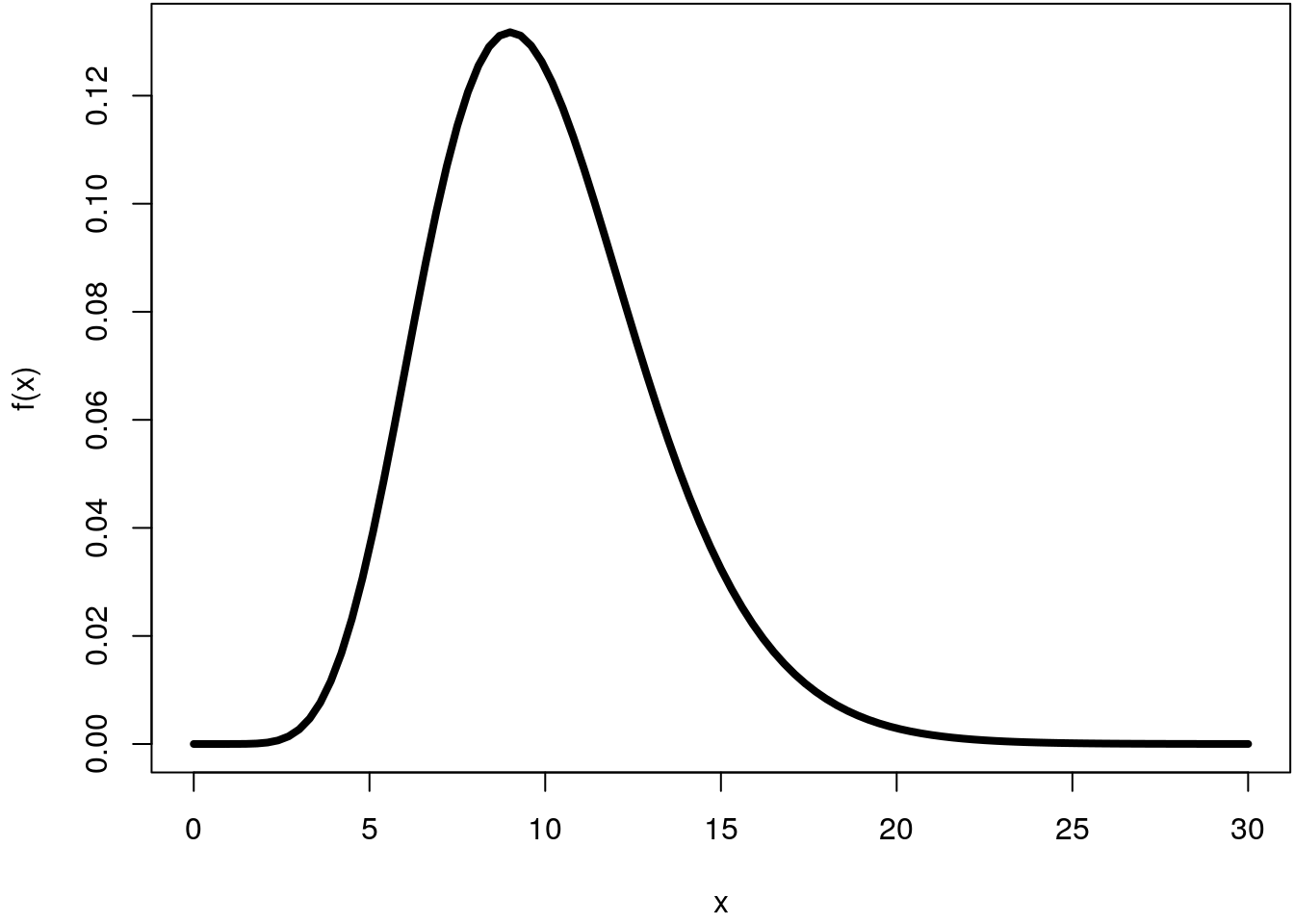

This integral can be computed using the cumulative distribution function (CDF) of the Gamma distribution and gives

pgamma(30, shape = 10) - pgamma(0, shape = 10)

## [1] 0.9999929

and results not too surprisingly nearly \(1\).

To compute the integral using simulation we need to define a rectangle that encloses the density function, e.g., with

par(mar = c(4.1, 4.1, 0.1, 0.1))
curve(f, 0, 30, ylim = c(0, 0.15), lwd = 4)
rect(0, 0, 30, 0.15, border = 4, lwd = 4)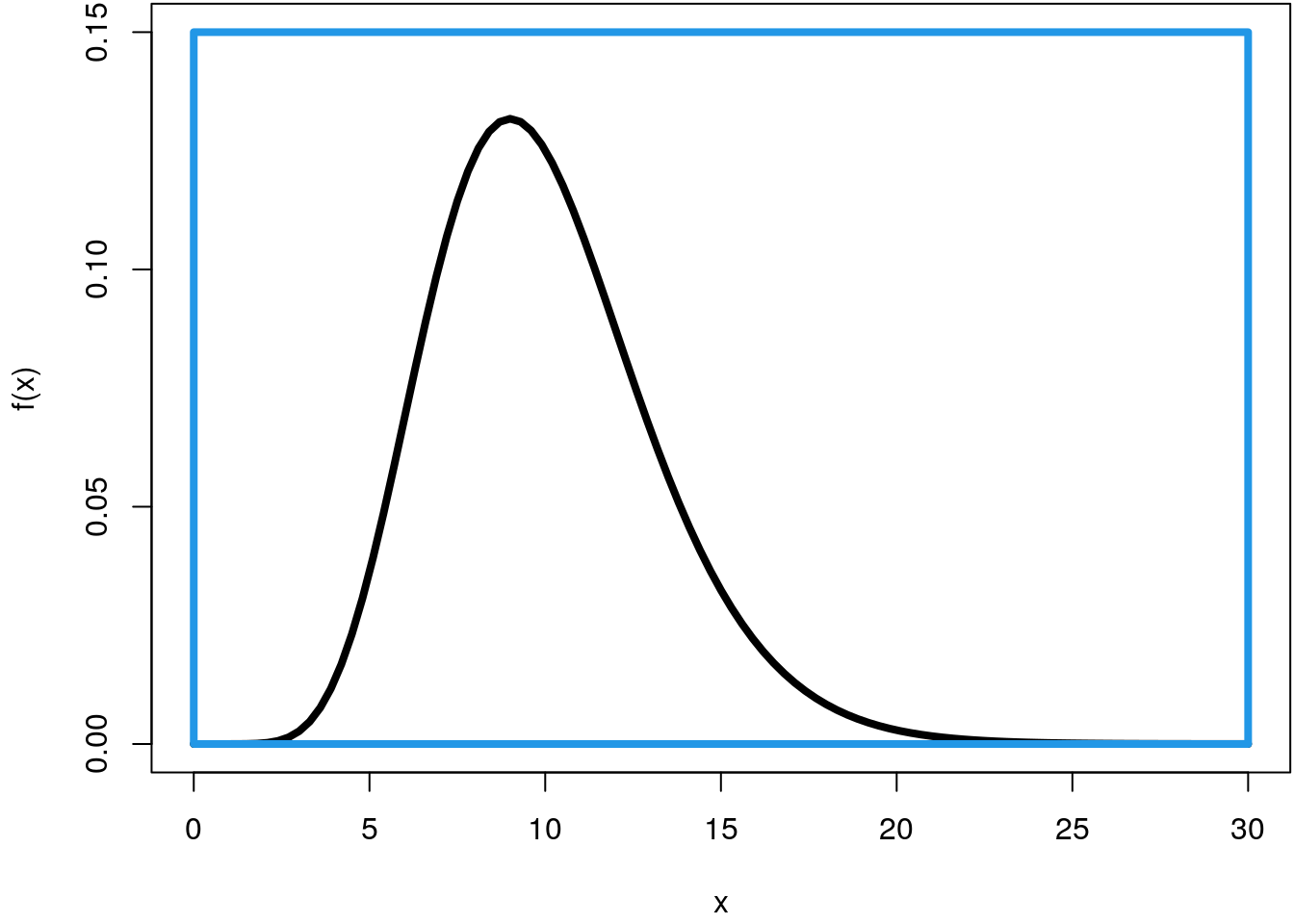

Now, we can easily draw random points within this rectangle using the runif() function, let’s sample \(200\) points for the moment and color each point that lies below the density curve in red.

## Set the seed for reproducibility.
set.seed(123)

par(mar = c(4.1, 4.1, 0.1, 0.1))
curve(f, 0, 30, ylim = c(0, 0.15), lwd = 4)
rect(0, 0, 30, 0.15, border = 4, lwd = 4)
n <- 200
p <- data.frame("x" = runif(n, 0, 30), "y" = runif(n, 0, 0.15))
fx <- f(p$x)
col <- rep(1, n)
col[p$y <= fx] <- 2
points(p, col = col)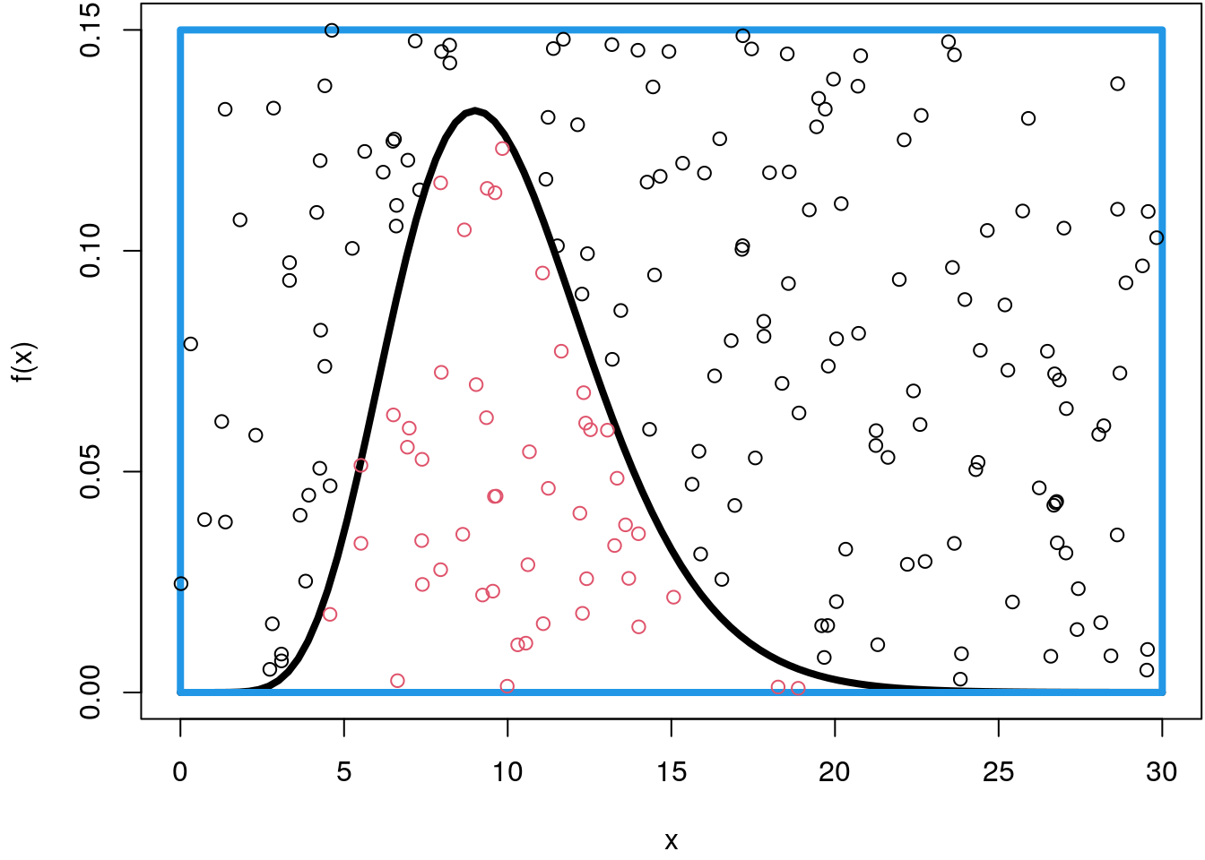

In order to approximate the integral by simulation, we only need the ratio of points that lie below the density function and scale it with the area of the rectangle \(30 \cdot 0.15 = 4.5\)

mean(p$y <= fx) * (30 * 0.15)

## [1] 1.1025

Ok, this is a very rough approximation since the integral should be very close to \(1\). If we use numerical integration as implemented in the integrate() function we get

integrate(f, 0, 30)

## 0.9999929 with absolute error < 2.1e-06

However, when sampling more data points, e.g., \(10000\) we get pretty close

## Set the seed for reproducibility.
set.seed(123)

par(mar = c(4.1, 4.1, 0.1, 0.1))
curve(f, 0, 30, ylim = c(0, 0.15), lwd = 4)
rect(0, 0, 30, 0.15, border = 4, lwd = 4)
n <- 10000
p <- data.frame("x" = runif(n, 0, 30), "y" = runif(n, 0, 0.15))
fx <- f(p$x)
col <- rep(1, n)
col[p$y <= fx] <- 2
points(p, col = col)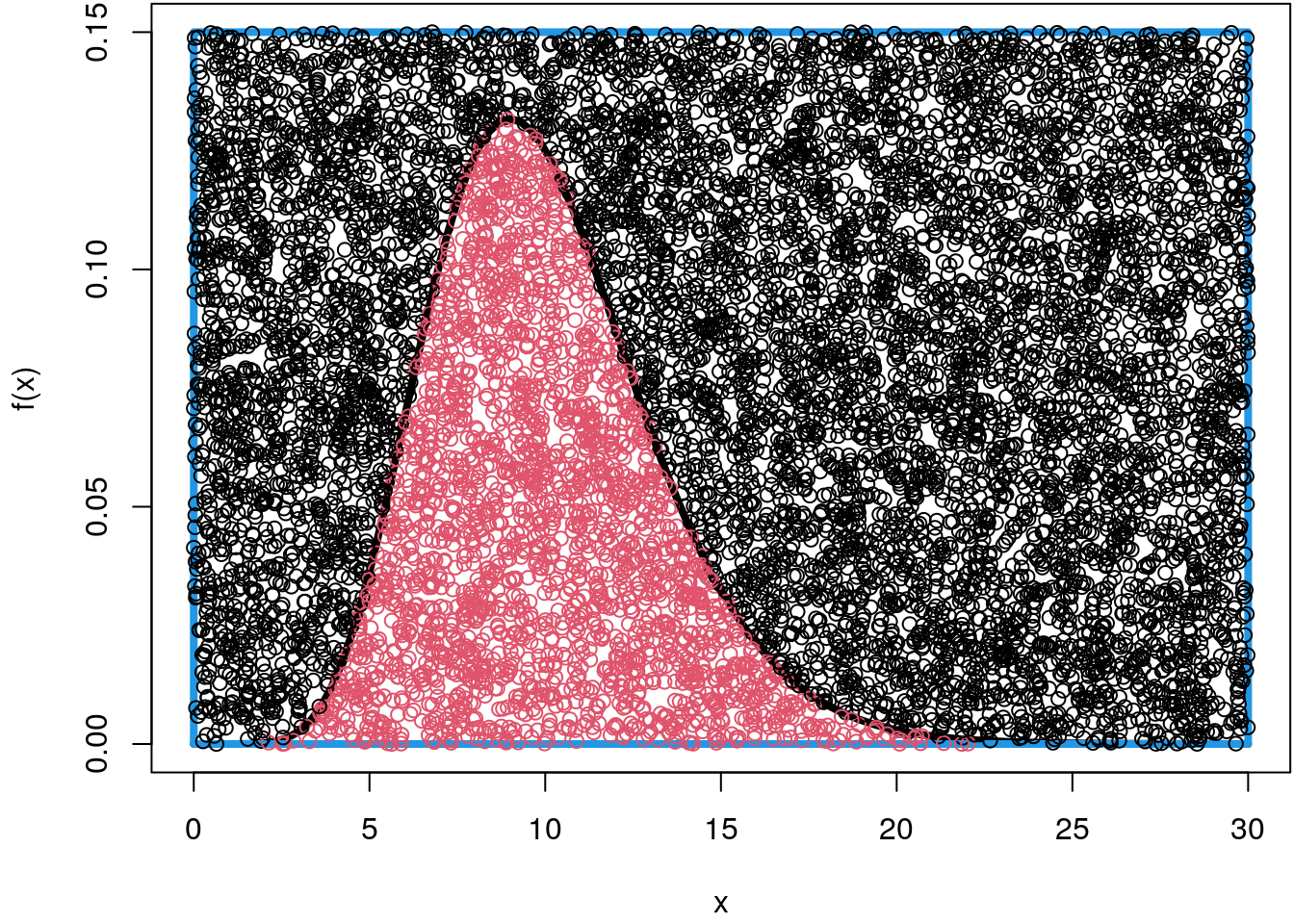

## Compute the integral.
mean(p$y <= fx) * (30 * 0.15)

## [1] 1.0287

More interestingly for us is the fact that we indeed sampled random numbers from the Gamma distribution with shape = 10 within the interval \([0, 30]\). To see this, we just need to drop all points that are above the density function and only save the position of the x-coordinate

## Extract the samples saving only
## the x-coordinate of the points.
x <- p[p$y <= fx, ]$x

## Draw a histogram.
par(mar = c(4.1, 4.1, 4.1, 0.1))
hist(x, freq = FALSE, ylim = c(0, 0.15), breaks = "Scott")

## Add the true density curve.
curve(f, 0, 30, add = TRUE, col = 2, lwd = 4)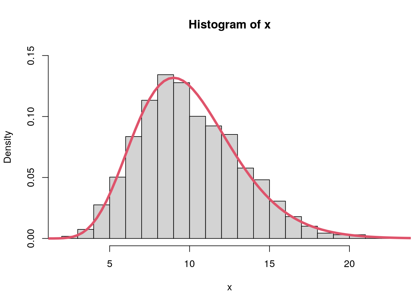

And indeed, the histogram clearly follows a gamma distribution with shape = 10 and rate = 1.

If these are true samples from the Gamma distribution, it is easy to compute for example the mean of this distribution

mean(x)

## [1] 10.0211

So this is very close to the true mean of \(10\). Again, let’s compare this using numerical integration

integrate(function(x) f(x) * x, -Inf, Inf)

## 10 with absolute error < 9.2e-07

Of course we could have drawn the gamma distributed random numbers directly via the inversion method, but that is not the point, for more complex Bayesian regression models we need a general method to draw random numbers from general distributions.

Exercise 6.1 Compute the mean, the 5% and 95% quantile using Monte Carlo integration of the following mixture distribution \[ f(x) = 0.4 \cdot N(\mu = -1, \sigma^2 = 1)(x) + 0.6 \cdot Ga(\alpha = 6, \beta = 1)(x), \] where \(\alpha\) is the shape parameter and \(\beta\) the rate of the Gamma distribution.

First, we need to setup the mixture density function and plot within a certain interval, let’s say within \([-10, 20]\)

f <- function(x) {
  0.4 * dnorm(x, mean = -1, sd = 1) + 0.6 * dgamma(x, shape = 6, rate = 1)
}

par(mar = c(4.1, 4.1, 0.1, 0.1))
curve(f, -10, 20, lwd = 4)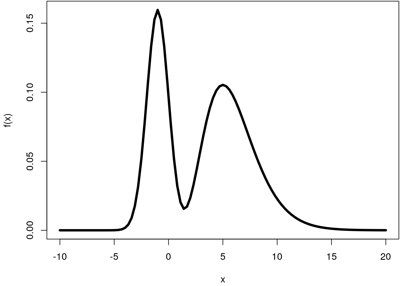

For simulation of this density using the Monte Carlo method, we need to define a rectangle that encloses the density curve.

par(mar = c(4.1, 4.1, 0.1, 0.1))
curve(f, -10, 20, lwd = 4, ylim = c(0, 0.2))
rect(-10, 0, 20, 0.2, border = 4, lwd = 4)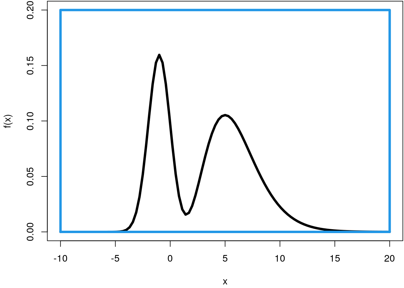

Now, we simulate from the mixture density the same way we did in the above example. However, to be relative precise we draw \(100000\) samples instead.

## Set the seed for reproducibility.
set.seed(123)

par(mar = c(4.1, 4.1, 0.1, 0.1))
curve(f, -10, 20, ylim = c(0, 0.2), lwd = 4)
rect(-10, 0, 20, 0.2, border = 4, lwd = 4)

## Draw points under the curve.
n <- 100000
p <- data.frame("x" = runif(n, -10, 20), "y" = runif(n, 0, 0.2))
fx <- f(p$x)
col <- rep(1, n)
col[p$y <= fx] <- 2
points(p, col = col)

## Only save the x-coordinate.
x <- p[p$y <= fx, ]$x

## Compute the mean and compare to integrate().
mean(x)

## [1] 3.205726

integrate(function(x) f(x) * x, -Inf, Inf)

## 3.2 with absolute error < 2.4e-05

## Compute the quantiles.
qx <- quantile(x, prob = c(0.05, 0.95))
print(qx)

##        5%       95% 
## -2.129017  9.612942

## Add to the plot.
abline(v = qx, col = 3, lwd = 2)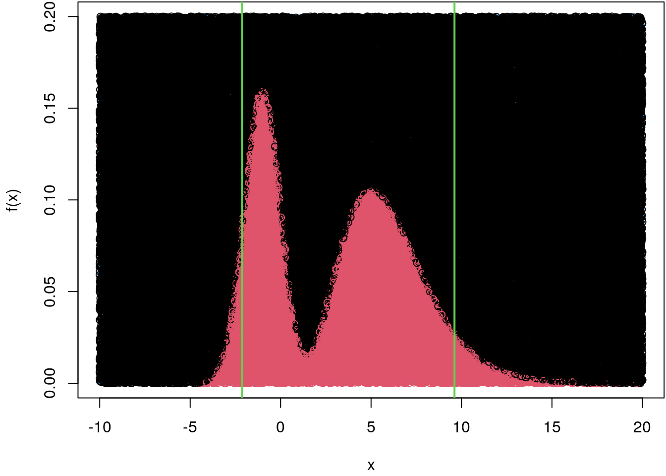

As we can see, this method works really well, but there are some significant drawbacks, which are explained in the following.

Rejection sampling

The reader will have noticed that the Monte Carlo sampling method for drawing random numbers from general distributions has limitations. For example, we had to specify interval limits in the previous section to construct the rectangle for this method, i.e. the calculation of an indefinite integral and thus the exact generation of random numbers is not possible.

With the rejection sampling method we avoid this problem by simply drawing points from a known distribution from which we can easily generate random numbers (inversion method) instead of drawing points from a rectangle.

The only thing we have to keep in mind is that the distribution from which we originally draw encloses the target distribution, just as was previously the case with the Monte Carlo method using the rectangle. Formally, the idea is to draw \(x\) from known distribution \(f_Y(x)\) instead of the target distribution \(f_X(x)\) directly, where there must be a \(\nu\) with \(0 < \nu < 1\), so that \(\nu f_X(x) \leq f_Y(x)\) for all \(x \in \mbox{supp}(X)\). This condition ensures that \(f_Y(x)\) is an envelope distribution. Then accept \(x\) as a random number drawn from \(f_X(x)\) with acceptance probability \[ \alpha(x) = \nu \cdot \frac{f_X(x)}{f_Y(x)}. \] Note that \(\nu\) is the probability of taking a sample. The larger \(\nu\) the better. Note that this similar as using Monte Carlo integration when we just looked if the sampled height, the y-coordinate, is under the density curve we want to sample from.

Univariate example

Let’s again pick the example from the last section and draw samples from a Gamma distribution with shape = 10 and rate = 1 (the default). To implement the rejection sampler we use the normal distribution with \(\mu = 10\) and \(\sigma^2 = 25\) as an envelope distribution and set \(\nu = 0.5\).

## The Gamma distribution we want to draw from.
f <- function(x) dgamma(x, shape = 10)

## The nu-scaled version.
fxnu <- function(x, nu = 0.5) nu * f(x)

par(mar = c(4.1, 4.1, 0.1, 0.1))
curve(fxnu, 0, 30, lwd = 4, ylim = c(0, 0.08))

## The envelope distribution.
f_Y <- function(x) dnorm(x, mean = 10, sd = 5)

## Add to plot.
curve(f_Y, 0, 30, col = 4, lwd = 4, add = TRUE)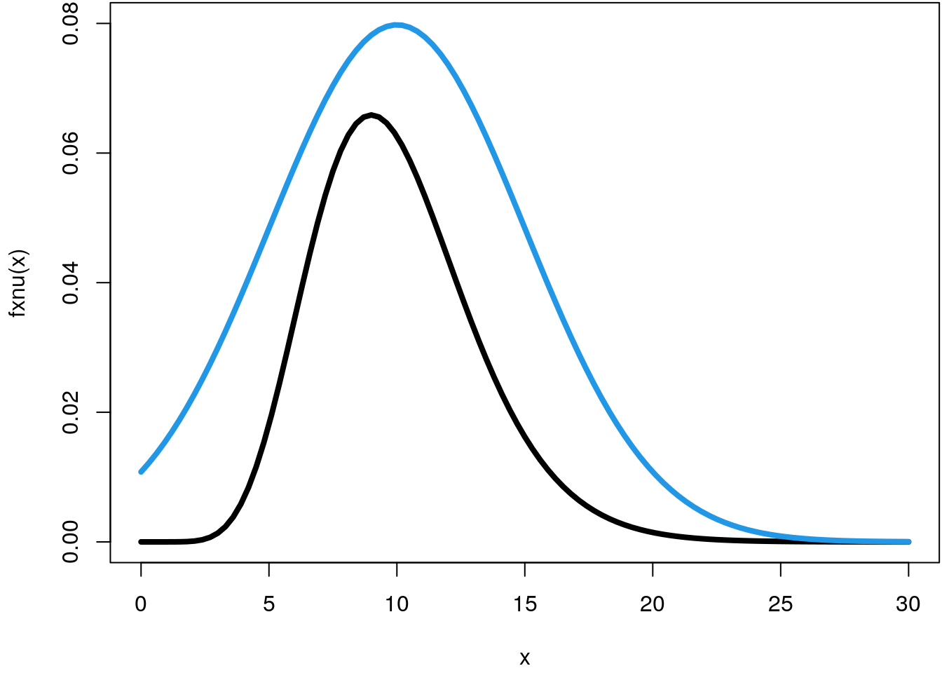

The algorithm can be implemented with

## The rejection sampler function.
rsamp <- function(n, f_X, f_Y, q_Y, nu)
{
  x <- rep(NA, length = n)
  i <- 0
  while(i < n) {
    y <- q_Y(runif(1))
    alpha <- nu * f_X(y) / f_Y(y) 
    u <- runif(1)
    if(u <= alpha) {
      i <- i + 1
      x[i] <- y
    }
  }
  return(x)
}

## Quantile function of the envelope distribution to
## draw samples using the inversion method.
q_Y <- function(p) qnorm(p, mean = 10, sd = 5)

## Draw 10000 samples.
set.seed(123)
x <- rsamp(10000, f_X = f, f_Y = f_Y, q_Y = q_Y, nu = 0.5)

## And plot the histogram.
hist(x, freq = FALSE, breaks = "Scott", ylim = c(0, 0.15))
curve(f, 0, 30, lwd = 4, col = 2, add = TRUE)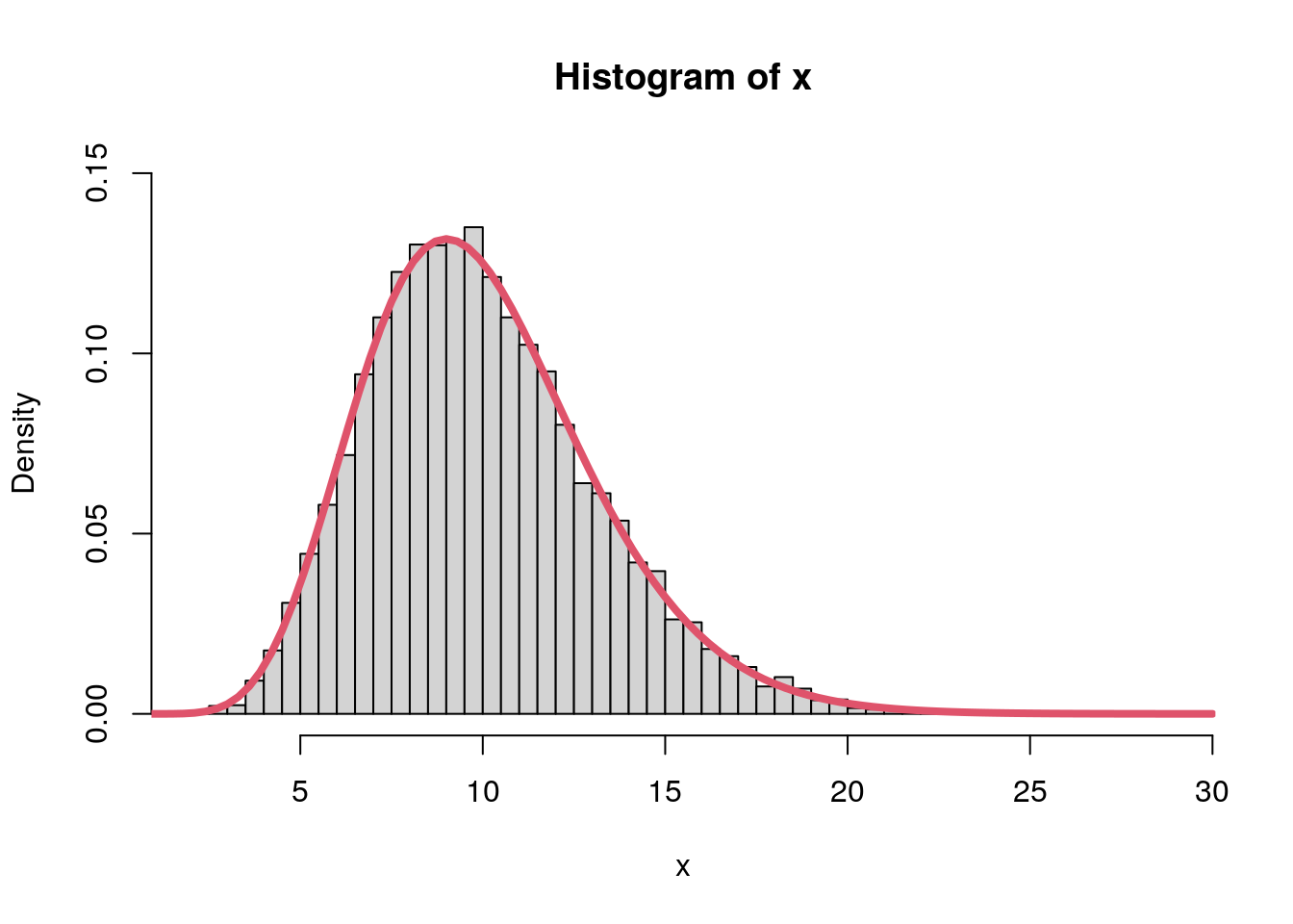

The rejection sampler apparently worked very well, compared to the Monte Carlo method we can actually generate random numbers for arbitrary distributions without having to determine interval limits in advance.

Linear model example

This example illustrates the rejection sampling method for the Bayesian linear model. We simulate a nonlinear relationship with \[ y = 1.2 + sin(x) + \varepsilon \] and \(\varepsilon \sim N(0, 0.3^2)\).

set.seed(123)

n <- 300

x <- runif(n, -2 * pi, 2 * pi)
y <- 1.2 + sin(x) + rnorm(n, sd = 0.3)

par(mar = c(4.1, 4.1, 0.1, 0.1))
plot(x, y)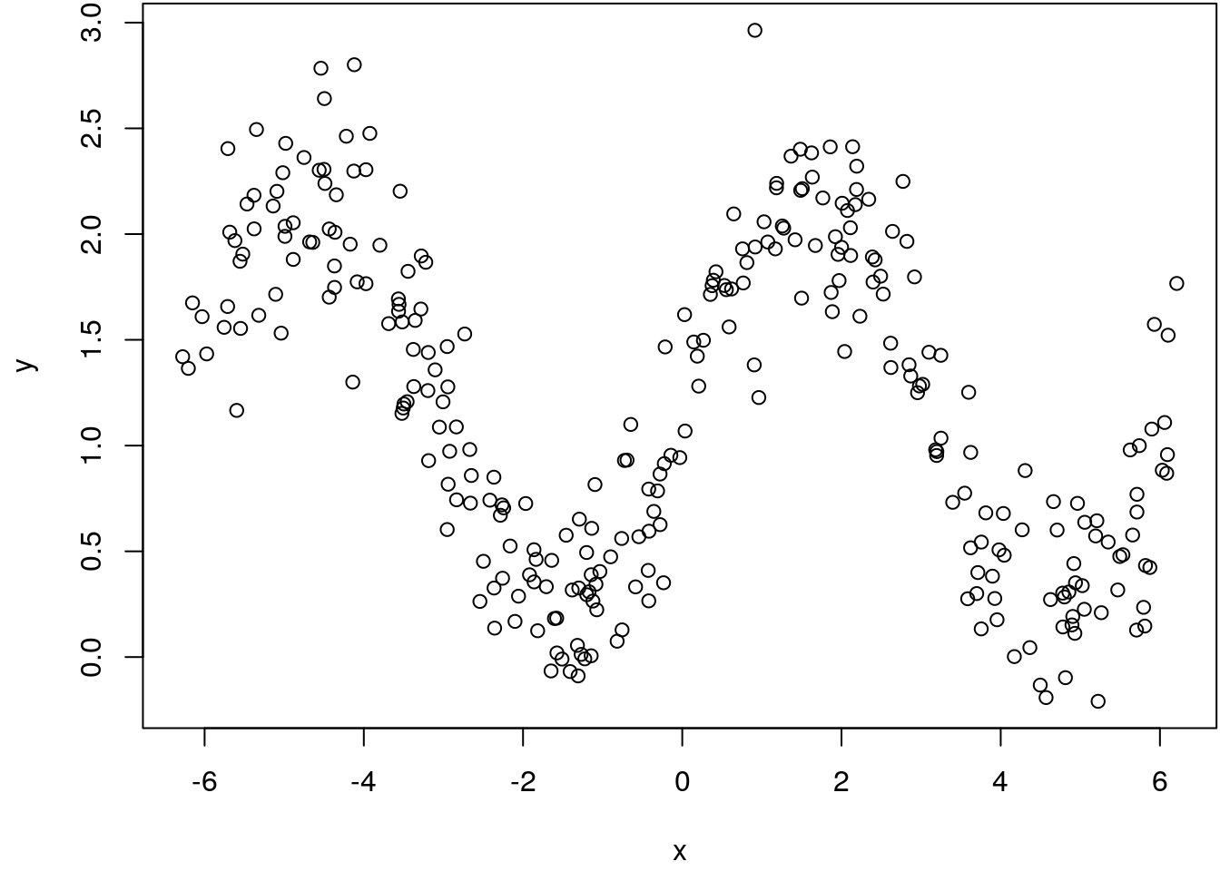

To set up the sampler for the Bayesian linear model we assign a vague normal prior on the regression coefficients \(\boldsymbol{\beta}\). Moreover, we work with the log-densities which is numerically much more stable. The log-posterior can be set up with

loglik <- function(theta) {
  eta <- X %*% theta
  sum(dnorm(y, mean = eta, sd = 0.3, log = TRUE))
}

logprior <- function(theta) {
  sum(dnorm(theta, mean = 0, sd = 1000, log = TRUE))
}

logpost <- function(theta) {
  loglik(theta) + logprior(theta)
}

Now, we set up the design matrix \(\mathbf{X}\) using orthogonal polynomials and specify the scaling parameter \(\nu\) of the rejection sampler. The algorithm runs for \(100000\) iterations.

## Design matrix.
X <- cbind(1, poly(x,8))
k <- ncol(X)

## Rejection sampler scaling parameter.
nu <- 0.3

## Number of iterations.
iter <- 100000

## Matrix to save the samples.
theta.save <- matrix(NA, iter, k)

## Initial values.
theta <- rep(0, k)

for(i in 1:iter) {
  ## Propose from envelop density.
  theta.prop <- rnorm(k, mean = theta, sd = 4)

  ## Compute acceptance rate (log scale).
  alpha <- log(nu) + logpost(theta.prop) - sum(dnorm(y, mean = theta, sd = 4, log = TRUE))

  ## Acceptance step.
  u <- runif(1)
  if(u <= min(c(exp(alpha), 1))) {
    theta.save[i, ] <- theta.prop
    theta <- theta.prop
  }

}

## Omit all NAs, i.e., unsuccessful draws.
theta.save <- na.omit(theta.save)

## Final number of saved samples.
print(dim(theta.save))

## [1] 1480    9

## Evaluate the regression curve for each sample.
fit <- apply(theta.save, 1, function(beta) {
  drop(X %*% beta)
})

## Compute quantiles from samples.
fit <- t(apply(fit, 1, quantile, probs = c(0.1, 0.5, 0.9), na.rm = TRUE))

## Plot the estimate.
par(mar = c(4.1, 4.1, 0.1, 0.1))
i <- order(x)
matplot(x[i], fit[i, ], type = "l", lty = c(2, 1, 2), col = 2, lwd = 2,
  xlab = "x", ylab = "f(x)")
points(x, y)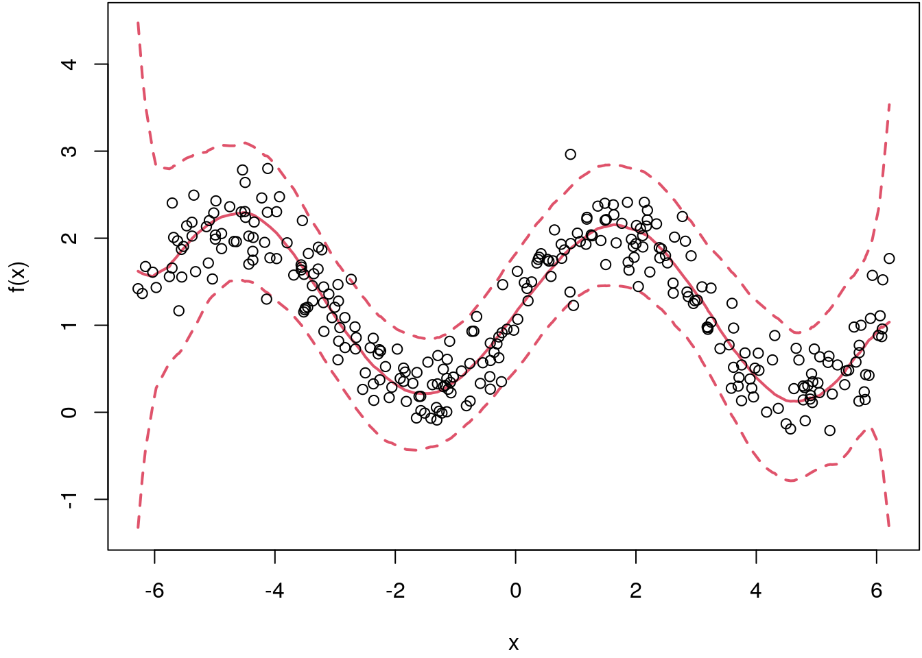

This seemed to work quite well, however, we only obtained \(1480\) samples although we used \(100000\) iterations of the algorithm. Hence, the acceptance rate is relatively low at \(1.48\)%. Also, the standard deviation of the envelop density is crucial, if it is too low or too high the sampler will always reject.

This behaviour already shows a little bit the limits of this method, especially if we remember that we want to estimate much more complex models with much more parameters. Rejection sampling quickly reaches its limits here, so we need more efficient methods to draw random numbers from the posterior density. The reason is that the probability of rejection increases exponentially as a function of the number of parameters.

Metropolis-Hastings Markov chain Monte Carlo

In the previous chapters we have shown how to draw random numbers from the posterior distribution. However, for complex Bayesian models with many parameters these methods are of limited use.

Fortunately, there is a class of algorithms, so called Marcov Chain Monte Carlo (MCMC) algorithms, which work in practice even for very large dimensions for the parameter of interest, vector \(\boldsymbol{\theta}\). In the following we will outline the basic principles of this method.

Markov chains

Before we explain the actual algorithm we first have to deal with the concept of a Markov chain. The samplers we have shown in the previous sections all generated i.i.d. random variables from the posterior distribution. In MCMC the samples are not i.i.d. anymore. The reason is that we construct a sample chain that moves should move over around the posterior distribution, i.e., the chain should explore all features of the target distribution. To really implement this, these Markov chains must have certain properties, otherwise we cannot draw random variables from the target distribution.

A Markov chain \(\left\{\theta^{[t]}\right\}\) is a sequence of dependent random variables \[ \theta^{[0]}, \theta^{[1]}, \theta^{[2]}, \ldots, \theta^{[t]}, \ldots \] such that the probability distribution \(\theta^{[t]}\) given the past variables depends only on \(\theta^{[t - 1]}\).

This conditional probability distribution is called transition kernel or Markov kernel \(K(\cdot, \cdot)\), that is \[ \theta^{[t + 1]} | \theta^{[0]}, \theta^{[1]}, \theta^{[2]}, \dots, \theta^{[t]} \sim K\left(\theta^{[t]}, \theta^{[t + 1]}\right). \]

For example, a simple random walk kernel satisfies \[ \theta^{[t + 1]} = \theta^{[t]} + \varepsilon_t, \] where \(\varepsilon_t \sim N(0, 1)\), independently of \(\theta^{[t]}\). Therefore, the Markov kernel \(K\left(\theta^{[t]}, \theta^{[t + 1]}\right)\) corresponds to a \(N\left(\theta^{[t]}, 1\right)\) density.

Metropolis-Hastings algorithm

For sampling from the posterior distribution we must construct a transition kernel that has the target distribution as its stationary distribution. This means, as the number of iterations increases we sample \(\boldsymbol{\theta}^{[t + 1]} \sim p(\boldsymbol{\theta}^{[t]} | \mathbf{y})\).

But how to set up such an transition kernel? Similar to rejection sampling we will use a proposal density where it is easy to sample of (in principle, the choice of the proposal density is arbitrary), but instead of scaling down the target posterior distribution, we compare how likely a newly proposed \(\boldsymbol{\theta}^*\) is compared to \(\boldsymbol{\theta}^{[t]}\). This is called the Metropolis-Hastings (MH, Hastings (1970)) acceptance probability and is computed by \[ \alpha(\boldsymbol{\theta}^* | \boldsymbol{\theta}^{[t]}) = \min \left\{ \frac{p(\boldsymbol{\theta}^* | \mathbf{y}) Q(\boldsymbol{\theta}^{[t]} | \boldsymbol{\theta}^*)} {p(\boldsymbol{\theta}^{[t]} | \mathbf{y}) Q(\boldsymbol{\theta}^* | \boldsymbol{\theta}^{[t]}) } ,1 \right\}. \] If the proposed \(\boldsymbol{\theta}^*\) is accepted, then the next state is \(\boldsymbol{\theta}^{[t + 1]} = \boldsymbol{\theta}^{*}\), otherwise \(\boldsymbol{\theta}^{[t + 1]} = \boldsymbol{\theta}^{[t]}\). The mechanism of the acceptance probability is comparably simple: If the newly proposed \(\boldsymbol{\theta}^*\) is in a region of the posterior with high probability mass compared to \(\boldsymbol{\theta}^{[t]}\), then the posterior ratio is \(\geq 1\). Secondly, we need to look at the proposal density ratio \(Q(\boldsymbol{\theta}^{[t]} | \boldsymbol{\theta}^{*}) / Q(\boldsymbol{\theta}^{*} | \boldsymbol{\theta}^{[t]})\). This term accounts for any biases that the proposal distribution might induce, i.e., if the current state had actually been \(\boldsymbol{\theta}^*\), what is the probability that you would have generated \(\boldsymbol{\theta}^{[t]}\) as the candidate value. This means that proposals are only accepted with high probability, if the chain is moving in regions of high probability mass of the posterior distribution. This so constructed Markov kernel guarantees that we will sample after some iterations from the posterior. This is also called the burn-in phase of a MCMC sampler.

Moreover, the density \(p(\boldsymbol{\theta} | \mathbf{y})\) does not appear directly in \(\alpha(\boldsymbol{\theta}^* | \boldsymbol{\theta}^{[t]})\), but only the ratio \(p(\boldsymbol{\theta}^* | \mathbf{y}) / p(\boldsymbol{\theta}^{[t]} | \mathbf{y})\). Therefore, all expressions in \(p(\boldsymbol{\theta} | \mathbf{y})\) that are constant can be omitted, i.e., the normalizing constant of the posterior is not needed. This is one of the big advantages of MCMC methods compared to conventional methods for drawing random numbers.

Note that the MH algorithm simplifies for symmetric proposals with \(Q(\boldsymbol{\theta}^* | \boldsymbol{\theta}^{[t]}) = Q(\boldsymbol{\theta}^{[t]} | \boldsymbol{\theta}^*)\). The acceptance probability then becomes \[ \alpha(\boldsymbol{\theta}^*|\boldsymbol{\theta}^{[t]}) = \min \left\{ \frac{p(\boldsymbol{\theta}^* | \mathbf{y})}{p(\boldsymbol{\theta}^{[t]} | \mathbf{y})} , 1 \right\}. \]

Although any proposal density will ultimately deliver samples from the posterior, it is important to choose appropriate proposal densities. In particular, acceptance probabilities should be large enough and correlation between successive iterates should be small. The smaller the correlation, the smaller is the required sample size to estimate characteristics of the posterior.

6.2.0.1 MH-sampler for the mean and variance for normal data

Let’s illustrate the MH sampler on a small example. In this exercise we want to compute parameter estimates for the mean and the variance using the following model:

The posterior of this model is given by \[ p(\boldsymbol{\theta} | \mathbf{y}) \propto p(\mathbf{y} | \mu, \sigma^2) p(\mu) p(\sigma^2). \]
The likelihood is \[ p(\mathbf{y} | \mu, \sigma^2) = \frac{1}{(2\pi\sigma^2)^{n/2}} \exp \left(-\frac{1}{2\sigma^2}(\mathbf{y} - \mathbf{1}\mu)^\top(\mathbf{y} - \mathbf{1}\mu)\right) \]
Similar the prior for \(\mu\) \[ p(\mu) = \frac{1}{(2\pi M_0)^{1/2}} \exp \left(-\frac{1}{2M_0}(\mu - m_0)^2\right). \]
For the \(\sigma^2\) prior, we use the inverse gamma distribution with \[ p(\sigma) = \frac{b^a}{\Gamma(a)} (\sigma)^{-(a + 1)} \exp(-b / \sigma). \]

In inverse Gamma prior is a commonly used prior for variances since the support is \(x \in (0, \infty)\). The following illustrates the inverse Gamma distribution for a couple of specifications of the hyperparameters \(a\) and \(b\).

igamma <- function(x, a = 2, b = 1) {
  b^a / gamma(a) * x^(-(a + 1)) * exp(-b / x)
}
par(mar = c(4.1, 4.1, 0.1, 0.1))
curve(igamma(x, a = 2, b = 1), 0, 10, lty = 2, ylab = "Density", n = 200)
curve(igamma(x, a = 1, b = 0.5), 0, 10, lty = 4, add = TRUE, n = 200)
curve(igamma(x, a = 1, b = 1), 0, 10, lty = 1, add = TRUE, n = 200)
curve(igamma(x, a = 0.5, b = 1), 0, 10, lty = 3, add = TRUE, n = 200)
curve(igamma(x, a = 0.0001, b = 0.0001), 0, 10, col = 2, lwd = 2,
  lty = 1, add = TRUE, n = 200)
legend("topright", c("a = 1, b = 1", "a = 2, b = 1",
  "a = 0.5, b = 1", "a = 1, b = 0.5", "a = 0.001, b = 0.001"),
  lwd = 1, lty = c(1:4, 1), col = c(rep(1, 4), 2), bty = "n")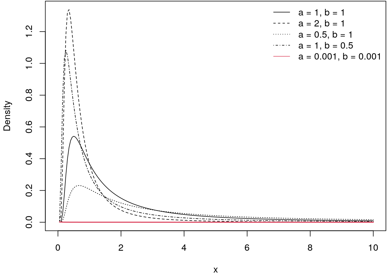

The distribution is highly right-skewed, hence, very large values for variances are not very likely. However if the hyper-parameters are set to \(a = 0.001\) and \(b = 0.001\) we again obtain a quasi non-informative (uniform) prior. This can also be seen by the red line, which is basically a flat line in this illustration.

In addition we set:

The hyper-parameters of the prior distributions are set to \(m_0 = 0\), \(M_0 = 10\), \(a = 0.5\) and \(b = 1\), which corresponds to relative vague priors.
The proposal densities for \(\mu\) and \(\sigma\) are both normal with \[ \mu^* | \mu^{[t]} \sim N\left(\mu^{[t]}, 0.1^2\right) \] and \[ \sigma^* | \sigma^{[t]} \sim N\left(\sigma^{[t]}, 0.1^2\right). \]
For starting the sampler we set \(\mu^{[0]} = \bar{y}\) and \(\sigma^{2^{[0]}} = s_y^2\).

Let’s simulate \(100\) data points

set.seed(111)
n <- 100
y <- rnorm(n, mean = 3.44, sd = 0.9)

Now, we need to set up the log-posterior (again note we compute the log-priors, log- likelihood and log-posterior for numerical reasons)

## Log-prior for sigma.
log_prior_sigma <- function(theta, a = 0.001, b = 0.001) {
  log(igamma(theta[2], a, b))
}

## Log-prior for mu.
log_prior_mu <- function(theta, mu0 = 0, M0 = 10) {
  dnorm(theta[1], mean = mu0, sd = M0, log = TRUE)
}

## Log-likelihood.
log_lik <- function(y, theta) {
  sum(dnorm(y, mean = theta[1], sd = theta[2], log = TRUE))
}

## Log-posterior.
log_post <- function(y, theta) {
  log_lik(y, theta) + log_prior_mu(theta) + log_prior_sigma(theta)
}

What is still missing is the proposal function. We use the normal distribution here, i.e., a symmetric proposal so the computation of the acceptance probability is easier.

prop <- function(x) rnorm(length(x), mean = x, sd = 0.1)

Note that the standard deviation in the proposal is a tuning parameter, we will focus on this topic in the upcoming.

Finally, we can set up the sampler and run the MCMC simulation with \(10000\) iterations.

## Set the seed.
set.seed(111)

## Set starting values for the parameters.
theta <- theta_prop <- c(mean(y), sd(y))

## Number of iterations.
T <- 10000

## Matrices to save the samples and acceptance rates.
theta_samples <- matrix(0, T, 2)
acc_rate <- matrix(0, T, 2)

colnames(theta_samples) <- colnames(acc_rate) <- c("mu", "sigma")

## Start sampling.
for(i in 1:T) {
  ## Iterate over parameters.
  for(j in 1:2) {
    ## Propose new parameter.
    theta_prop[j] <- prop(theta[j])

    ## Compute acceptance probability.
    ## Note, as we compute the log-posterior, we need to use
    ## exp() to get this on to the probability scale.
    alpha <- exp(log_post(y, theta_prop) - log_post(y, theta))

    ## Acceptance step.
    if(!is.na(alpha) && runif(1) < min(alpha, 1)) {
      theta[j] <- theta_prop[j]
      acc_rate[i, j] <- 1
    }

    ## Save current parameter sample.
    theta_samples[i, j] <- theta[j]
  }
}

The sampling runtime is actually pretty fast. The first thing you usually do after sampling is to look at the trace plots and the ACF of the samples. Here we can easily see if the Markov chains are stationary and have converged against the target distribution.

par(mfrow = c(2, 2), mar = c(4.1, 4.3, 1.1, 1.1))
plot(theta_samples[, 1], type = "l", xlab = "Iteration", ylab = expression(mu))
acf(theta_samples[, 1], lag.max = 250, main = "")
plot(theta_samples[, 2], type = "l", xlab = "Iteration", ylab = expression(sigma))
acf(theta_samples[, 2], lag.max = 250, main = "")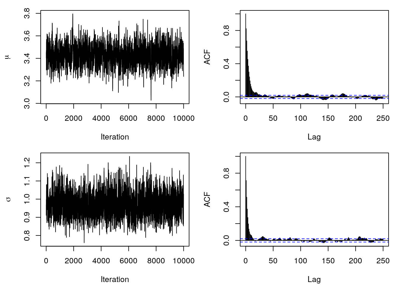

So this seemed to work out pretty nice. We can clearly see that both chains do not have a trend and it seems that we obtained i.i.d. samples from the posterior distribution, since the empirical ACF shows quite low autocorrelation already after lag 20. This is also reflected by the satisfying acceptance rates with

colMeans(acc_rate)

##     mu  sigma 
## 0.4904 0.4726

Now, we can easily compute posterior mean estimates as well as 95% credible intervals

t(apply(theta_samples, 2, function(x) {
  x <- c(
    quantile(x, prob = 0.025),
    mean(x),
    quantile(x, prob = 0.975)
  )
  names(x) <- c("2.5%", "Mean", "97.5%")
  x
}))

##           2.5%      Mean    97.5%
## mu    3.250141 3.4306809 3.621614
## sigma 0.849916 0.9688957 1.106319

Apparently the MCMC algorithm was able to estimate the true parameters of \(\mu = 3.44\) and \(\sigma = 0.9\) quite well from the data.

Now, let’s run the sampler again, but this time we use different starting values for the parameters.

theta <- theta_prop <- c(0, 2)

We use the same code as above and obtain the following parameter path.

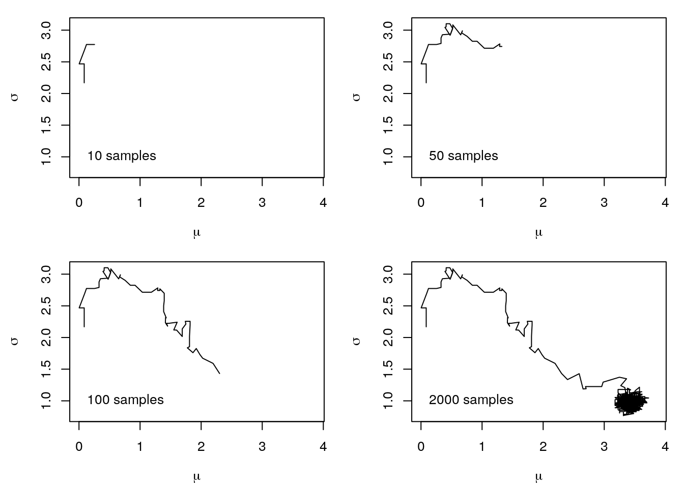
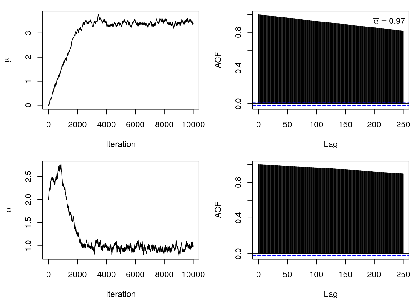
You can clearly see that the MCMC sampler now takes a little longer to get into the region of the true parameter values. This is the so-called burnin, i.e., we have to remove these samples to really only get samples from the right region before we can calculate any statistics of the parameters.

This behaviour of the Markov chains can easily be seen in the Traceplots and the ACF plot.

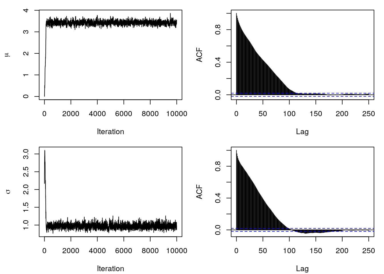
The plots show, that it took a little more than \(100\) iterations until the Markov chains reached stationarity and started generating samples from the posterior distribution. Hence, good starting values are essential, especially for more complicated problems. Moreover, so far we did not talk about hyper parameter tuning of the proposal functions. The problem is, if we set the standard deviation too low and we have poor starting values, the Markov chains may take very long until they reach the desired stationary regions, or they even get stuck at some point. In contrast, if the standard deviation is too large, if run into the risk that we will never accept any samples, because the proposed values are very likely to be in regions of the posterior with very low probability mass. This behavior is pretty much reflected by the acceptance rates, i.e., these are a good first indicator if everything went well. Together with the traceplots and ACF plots we can then judge if MCMC chains converged and we have i.i.d. samples of the posterior distribution.

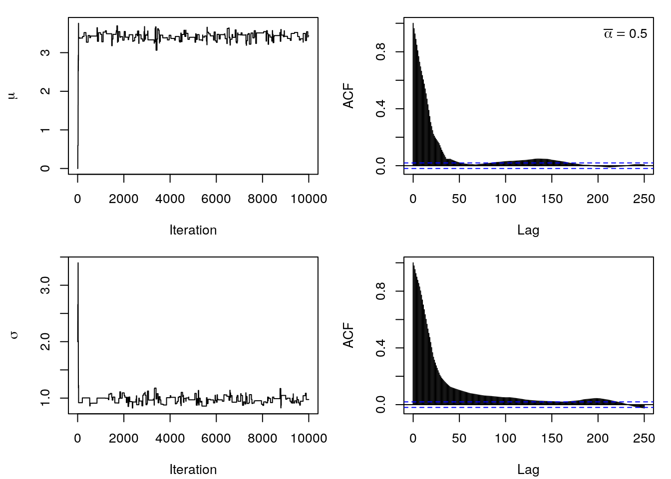
To end this example we first reduce the standard deviation of the proposal denstities to

prop <- function(x) x + rnorm(1, sd = 0.01)

and run the sampler again. This gives the following trace- and ACF plots.

It can be clearly seen that the Markov chains take a very long time to reach a stationary region. Additionally, the samples are anything but i.i.d., they show a very large autocorrelation. Therefore a high acceptance rate, here \(\bar{\alpha} = 0.97\), is not necessarily related to good samples from the posterior distribution.

Secondly, let’s increase the standard deviation of the proposals by

prop <- function(x) x + rnorm(1, sd = 0.8)

and again look at trace- and ACF plots.

The paths have a rather stepwise course, which means that many samples were simply not accepted. This is especially true for \(\sigma\), since we are drawing proposals from a normal distribution, it is of course possible that we may also generate negative values for \(\sigma\) from time to time. This leads to the log-likelihood outputting NA and not being accepted.

One way to work around the problem with positivity is to draw from the normal distribution, but then run the samples through the exp() function, which makes them always be positive.

Exercise 6.2 In the previous section we estimated a linear model using the rejection sampling method. In this exercise you should set up an MH-MCMC algorithm to estimate a linear model. The task is to provide posterior mean, 2.5% and 97.5% credible intervals in the Munich rent model \[ \texttt{rentsqm} = \beta_0 + f(\texttt{area}) + \varepsilon \] with \(\varepsilon \sim N(0, \sigma^2)\), for function \(f(\texttt{area})\) and the variance parameter \(\sigma^2\). The possibly nonlinear function \(f(\texttt{area})\) should be modeled using orthogonal polynomials of degree \(3\). Note that the regression coefficients should be sampled within one block.

To set up the sampler we adopt the model and the code from the above. The model is specified by:

The likelihood of the model is \[ p(\mathbf{y} | \boldsymbol{\beta}, \sigma^2) = \frac{1}{(2\pi\sigma^2)^{\frac{n}{2}}} \exp \left(-\frac{1}{2\sigma^2}(\mathbf{y} - \mathbf{X}\boldsymbol{\beta})^\top(\mathbf{y} - \mathbf{X}\boldsymbol{\beta})\right) \]
The priors are given as follows \[ \boldsymbol{\beta} \sim N(\mathbf{m}_0, \mathbf{M}_0) \] and \[ \sigma^2 \sim IG(a, b). \]

First, we need to load the data and setup the design matrix \(\mathbf{X}\).

load("data/MunichRent.rda")

## Set up design matrix including intercept.
X <- cbind(1, poly(MunichRent$area, 3))

## Save the number of regression coefficients beta.
k <- ncol(X)

## Now we can define priors, etc.
## Log-prior for sigma^2.
log_prior_sigma2 <- function(theta, a = 0.001, b = 0.001) {
  log(igamma(theta$sigma2, a, b))
}

## Log-prior for beta.
log_prior_beta <- function(theta, mu0 = 0, M0 = 10) {
  dnorm(theta$beta, mean = mu0, sd = M0, log = TRUE)
}

## Log-likelihood.
log_lik <- function(y, theta) {
  eta <- X %*% theta$beta
  sum(dnorm(y, mean = eta, sd = sqrt(theta$sigma2), log = TRUE))
}

## Log-posterior.
log_post <- function(y, theta) {
  log_lik(y, theta) + log_prior_beta(theta) + log_prior_sigma2(theta)
}

## Set the number of iterations.
T <- 100000

## Set initial values and matrices to save the samples
## and acceptance rates. As named lists also.
theta_samples <- list(
  "beta" = matrix(0, T, k),
  "sigma2" = matrix(0, T, 1)
)
acc_rate <- list(
  "beta" = rep(0, T),
  "sigma2" = rep(0, T)
)

## To ease sampling we define theta as a list,
## one entry for beta and one for sigma2.
theta <- list(
  "beta" = rep(0, k),
  "sigma2" = 1
)
theta_prop <- theta

## Proposal functions, also as list to account
## for better control using different standard
## deviation for the proposals.
prop <- list(
  "beta" = function(x) x + rnorm(length(x), sd = c(0.1, 0.2, 0.25, 0.15)),
  "sigma2" = function(x) x + rnorm(1, sd = 0.2)
)

## The response y is rentsqm.
y <- MunichRent$rentsqm

## Save the samples, since computing time can be quite long.
if(!file.exists("theta_samples.rda")) {
  ## Set the seed.
  set.seed(123)

  ## Start sampling.
  for(i in 1:T) {
    ## Iterate over parameters.
    for(j in c("beta", "sigma2")) {
      ## Propose new parameter.
      theta_prop[[j]] <- prop[[j]](theta[[j]])

      ## Compute acceptance probability.
      alpha <- exp(log_post(y, theta_prop) - log_post(y, theta))

      ## Acceptance step.
      if(!is.na(alpha) && runif(1) < min(alpha, 1)) {
        theta[[j]] <- theta_prop[[j]]
        acc_rate[[j]][i] <- 1
      }

      ## Save current parameter sample.
      theta_samples[[j]][i, ] <- theta[[j]]
    }
  }

  ## Save.
  save(theta_samples, file = "theta_samples.rda")
} else {
  load("theta_samples.rda")
}

## Show the trace- and ACF plots.
par(mfrow = c(5, 2), mar = c(4.1, 4.3, 1.1, 1.1))
for(j in 1:k) {
  plot(theta_samples$beta[, j], type = "l",
    xlab = "Iteration", ylab = parse(text = paste0("beta[", j, "]")))
  acf(theta_samples$beta[, j], lag.max = 250, main = "")
}
plot(theta_samples$sigma2, type = "l",
  xlab = "Iteration", ylab = expression(sigma^2))
  acf(theta_samples$sigma2, lag.max = 250, main = "")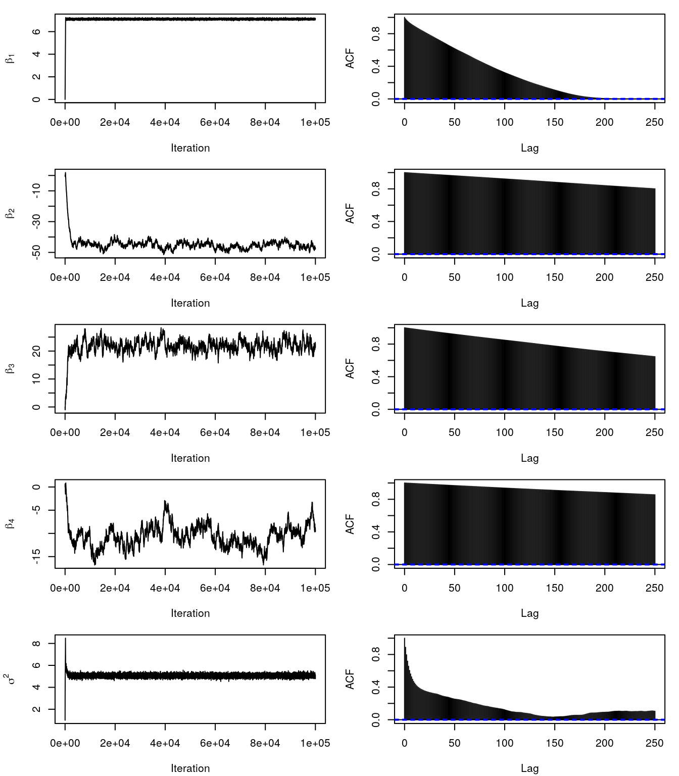

The trace- and ACF plots indicate that the Markov chains take quite long to converge. Moreover, the samples have very high autocorrelation. The reason is that the standard deviations of the proposals are not optimal. There is a way to get around this by tuning these in a learning phase, this is also called adaptive MH-MCMC. However, even careful tuning can be difficult for certain problems. We will see in the upcoming how we can sample from the posterior in the linear model and general smooth models much more efficiently. For the moment, we use another technique to obtain i.i.d. samples. We can do two things since we have produced quite a lot of samples: (1) withdraw the burnin phase, here approximately the first 20000 samples, and (2) thin the chains and only use 1000 samples, this is called the thinning parameter, which can be controled in most software implementations for MCMC.

for(j in c("beta", "sigma2")) {
  theta_samples[[j]] <- theta_samples[[j]][-c(1:20000), , drop = FALSE]
  take <- seq.int(1, nrow(theta_samples[[j]]), length = 1000)
  theta_samples[[j]] <- theta_samples[[j]][take, , drop = FALSE]
}

## Again show trace- and ACF plots.
par(mfrow = c(5, 2), mar = c(4.1, 4.3, 1.1, 1.1))
for(j in 1:k) {
  plot(theta_samples$beta[, j], type = "l",
    xlab = "Iteration", ylab = parse(text = paste0("beta[", j, "]")))
  acf(theta_samples$beta[, j], lag.max = 250, main = "")
}
plot(theta_samples$sigma2, type = "l",
  xlab = "Iteration", ylab = expression(sigma^2))
  acf(theta_samples$sigma2, lag.max = 250, main = "")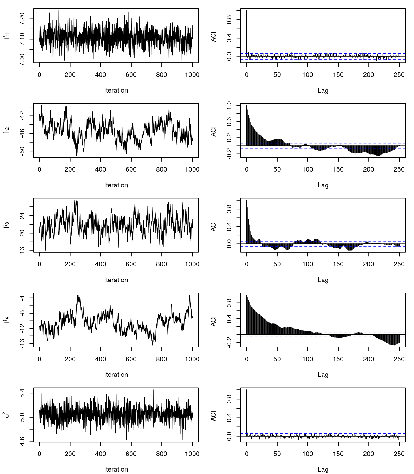

This still does not look perfect, however, we will use the samples to compute the posterior mean and 2.5% and the 97.5% credible intervals.

## Small helper function.
c95 <- function(x) {
  qx <- quantile(x, probs = c(0.025, 0.975), na.rm = TRUE)
  return(c(qx[1], Mean = mean(x, na.rm = TRUE), qx[2]))
}

## Compute effect of covariate area for each sample of beta.
fit <- apply(theta_samples$beta, 1, function(beta) {
  X %*% beta
})

fit <- t(apply(fit, 1, c95))

print(head(fit))

##          2.5%     Mean    97.5%
## [1,] 8.633755 8.796715 8.957431
## [2,] 6.016393 6.216198 6.380754
## [3,] 9.190784 9.439080 9.659319
## [4,] 8.293070 8.420882 8.556725
## [5,] 6.078040 6.248059 6.389248
## [6,] 6.853058 6.953255 7.048366

## Plot estimated effect.
par(mar = c(4.1, 4.1, 0.1, 0.1))
plot(rentsqm ~ area, data = MunichRent, col = rgb(0.1, 0.1, 0.1, alpha = 0.4))
i <- order(MunichRent$area)
matplot(MunichRent$area[i], fit[i, ], type = "l", lty = c(2, 1, 2),
  col = 2, lwd = c(1, 2, 1), add = TRUE)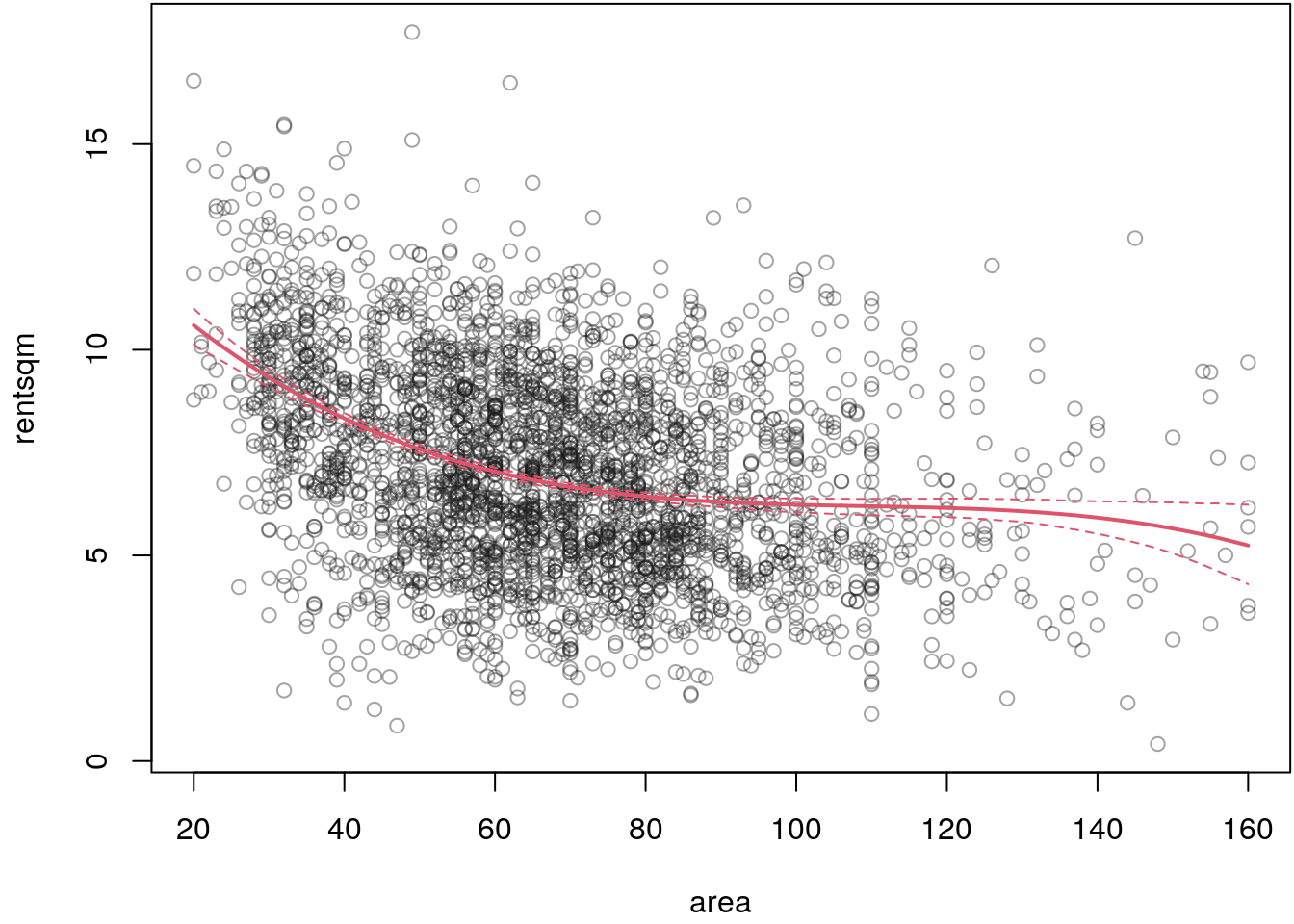

## Estimate for sigma2.
c95(theta_samples$sigma2)

##     2.5%     Mean    97.5% 
## 4.816749 5.055019 5.293146

The estimated effect of covariate area seems to be reasonable, although for a final model we would need to run the MCMC sampler even longer to obtain i.i.d. samples from the posterior distribution.

To sum up, the method of MH-MCMC is principally useful for very general Bayesian models. However, as already mentioned, it is quite difficult to get the hyper-parameters of the proposal densities right. There is some literature about adaptive versions of the sampler, but these are still not very convincing when wanting to estimate complex flexible regression models with thousands of parameters.

Slice MCMC

All MCMC methods dealt with so far have the disadvantage that one has to carefully turn several set screws in order to be able to cope with more complicated estimation problems. A particularly attractive method, and I will say right away that it is not suitable for all possible problems, is called slice sampling (Neal 2003).

Suppose you want to sample from an arbitrary density an univariate variable \(X \sim p(x)\) and further assume that it is impossible to sample from \(p(x)\) directly. The idea is to introduce an auxiliary variable \(U\) that allows us to explore \((X, U) \sim p(x, u)\) as our target density. By simple rules we may write \(p(x, u) = p(x)p(u|x)\) which leads to an auxiliary sampling strategy where we can first sample \(U\) and \(X\) afterwards.

The general sampling scheme with posterior density \(p(\boldsymbol{\theta}|\mathbf{y})\) is actually quite simple:

Sample \(h \sim \mathcal{U}(0, p(\theta_{j}^{[t]} | \, \cdot))\).
Sample \(\theta_{j}^{[t+1]} \sim \mathcal{U}(S)\) from the horizontal slice \(S = \{\theta_{j}: h < p(\theta_{j} | \, \cdot)\}\).

This means, given the current position \(\theta_{j}^{[t]}\) we need to evaluate the (log-) posterior to obtain the height of the function \(p(\theta_{j}^{[t]} | \, \cdot)\). Then we sample uniformly between \(0\) and \(p(\theta_{j}^{[t]} | \, \cdot)\) and obtain a vertical position \(h\). From this sampled height we then search for the edges of the target function. This step is computationally a little bit more involved. If we have the edges, we can easily sample a new position \(\theta_{j}^{[t+1]}\) uniformly on this slice.

Let’s illustrate this using R. To implement the slice sampler we need a function that finds the position of the edges of the target function given a position \(\theta_{j}^{[t]}\) and a height \(h\).

## Function to find edges.
## Argument x is the current position, target is the target function,
## height is the height where we need to find the edges, step is
## the steplength we go left and right of x to find the edges,
## eps is the relative error allowed for finding an edge.
find_edges <- function(x, target, height,
  step = 0.5, eps = 0.0001)
{
  ## Initial left and right edge.
  left <- right <- x

  ## Step size for both, left and right.
  step <- rep(step, length.out = 2)

  ## Search the left side.
  repeat {
    if((hs <- target(left)) <= height) {
      err <- abs((hs - height)/height)
      if(err <= eps) {
        break
      } else {
        left <- left + step[1]
        step[1] <- 0.95 * step[1]
      }
    }
    left <- left - step[1]
  }

  ## Search the right side.
  repeat {
    if((hs <- target(right)) <= height) {
      err <- abs((hs - height)/height)
      if(err <= eps) {
        break
      } else {
        right <- right - step[2]
        step[2] <- 0.95 * step[2]
      }
    }
    right <- right + step[2]
  }

  c(left, right)
}

## Test on complicated mixture distribution.
f <- function(x) {
  0.4 * dnorm(x, mean = -1, sd = 1) + 0.6 * dgamma(x, shape = 6, rate = 1)
}

## Find the edges.
edges <- find_edges(5, target = f, height = 0.05)

## Visualize.
par(mar = c(4.1, 4.1, 0.1, 0.1))
curve(f, -10, 20, lwd = 2, axes = FALSE, n = 500,
  xlab = "", ylab = expression(f(theta)))
points(edges[1], f(edges[1]), col = 2, pch = 16, cex = 1.2)
points(edges[2], f(edges[2]), col = 2, pch = 16, cex = 1.2)
lines(c(edges), f(edges), col = 2, lwd = 2)
lines(c(5, 5), c(0, 0.05), col = 4, lwd = 2)
points(c(5, 5), c(0, 0.05), col = 4, pch = 16, cex = 1.2)
axis(1, at = 5, label = expression(theta^(t)))
axis(2)
axis(1, at = c(-10, 0, 20))
box()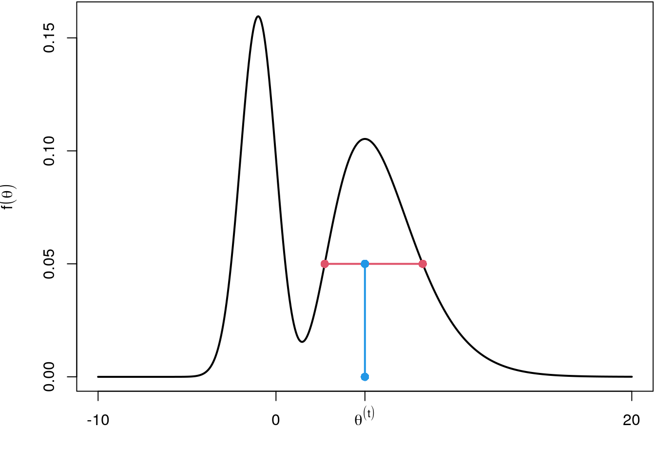

The find_edges() implementation is surely not the most efficient one but does the job for the moment. The red horizontal line defines the slice from which we can now sample a new position \(\theta^{[t+1]}\) using runif(). The complete slice sampler just needs a few lines of code.

## Slice sampling implementation.
## Argument n specifies the number of samples,
## target is the target function we want to sample from,
## start is a vector of initial starting positions,
## ... are passed to find_edges().
sliceMCMC <- function(n, target, start, ...) {
  ## Vector where we can save the samples.
  samples <- rep(NA, n)

  ## Set initial value.
  theta <- start

  ## Iterate n times.
  for(i in 1:n) {
    ## Draw the height.
    u <- runif(1, 0, target(theta))

    ## Find the edges.
    edges <- find_edges(theta, target, height = u, ...)

    ## Sample new position.
    theta <- runif(1, edges[1], edges[2])

    ## Save.
    samples[i] <- theta
  }

  return(samples)
}

## Test the slice sampling function.
set.seed(123)
x <- sliceMCMC(10000, target = f, start = 0, step = 1)

## Compare with true density.
hist(x, breaks = "Scott", freq = FALSE)
curve(f, min(x), max(x), add = TRUE, col = 2, lwd = 2, n = 500)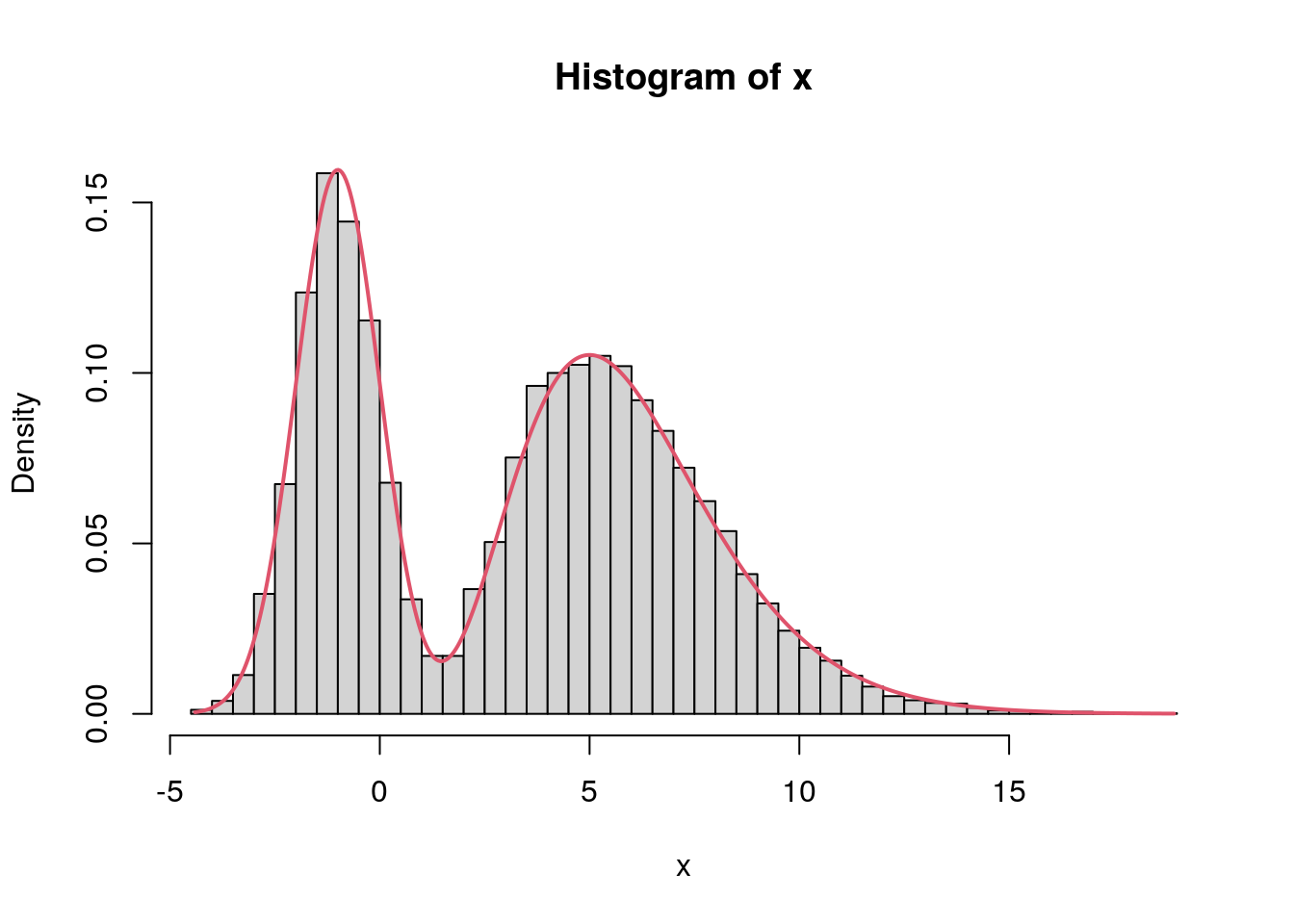

The slice sampler successfully sampled from the mixture distribution. The great advantage is, that we have 100% acceptance rates since we always sample uniformly under the target density. The con is that finding the edges can take some time in more complicated problems. We will use slice sampling in the upcoming when we need to sample multivariate shrinkage parameters for smooth function estimation.

Gibbs sampling

The MH-sampler and slice sampler are quite flexible tools for estimating Bayesian models, however, for large scale problems computational time is a disadvantage. Moreover, in MH-sampling mixing properties heavily depend on the choice of the scaling parameters of the proposal densities. The acceptance rates then become rather small even for well-designed MH algorithms, because a high-dimensional random number has to be accepted or not. In most cases no (simple) methods for directly drawing random numbers from the density \(p(\boldsymbol{\theta} | \mathbf{y})\) of the entire parameter vector are available.

Often, however, random numbers can be directly drawn from the conditional densities \(p(\boldsymbol{\theta}_1 | \cdot), p(\boldsymbol{\theta}_2 \, | \, \cdot ), \dots, p(\boldsymbol{\theta}_K | \cdot )\), where \(p(\boldsymbol{\theta}_k | \cdot)\) denotes the conditional density of \(\boldsymbol{\theta}_k\) given all other blocks \(\boldsymbol{\theta}_1, \dots, \boldsymbol{\theta}_{s - 1}, \boldsymbol{\theta}_{s + 1}, \dots, \boldsymbol{\theta}_{S}\) and the data \(\mathbf{y}\). These densities are called . Gibbs sampling consists in successively drawing random numbers from the full conditionals in each iteration and accepting them (with probability one, i.e., 100% acceptance) as the next state of the Markov chain. After a burn-in phase the sampled random numbers can be considered as realizations from the marginal posteriors \(p(\boldsymbol{\theta}_1 | \mathbf{y}), p(\boldsymbol{\theta}_2 | \mathbf{y}), \dots, p(\boldsymbol{\theta}_K | \mathbf{y})\).

To illustrate Gibbs sampling we set up the normal linear regression model \[ \mathbf{y} = \mathbf{X}\boldsymbol{\beta} + \boldsymbol{\varepsilon} \] with this method. For specifying the posterior we need the following:

The likelihood of the model is \[ p(\mathbf{y} | \mu, \sigma^2) = \frac{1}{(2\pi\sigma^2)^{\frac{n}{2}}} \exp \left(-\frac{1}{2\sigma^2}(\mathbf{y} - \mathbf{X}\boldsymbol{\beta})^\top(\mathbf{y} - \mathbf{X}\boldsymbol{\beta})\right) \]
The prior for \(\boldsymbol{\beta}\) is a joint prior with \[ p(\boldsymbol{\beta}, \sigma^2) = p(\boldsymbol{\beta} | \sigma^2)p(\sigma^2), \] where \[ \boldsymbol{\beta} | \sigma^2 \sim N(\mathbf{m}_0, \sigma^2\mathbf{M}_0), \,\,\, \sigma^2 \sim IG(a, b), \] \[\begin{eqnarray*} p(\boldsymbol{\beta}, \sigma^2) &=& \frac{1}{(2\pi)^{\frac{p}{2}}(\sigma^2)^{\frac{p}{2}}| \mathbf{M}_0|^{\frac{1}{2}}} \exp\left(- \frac{1}{2\sigma^2} (\boldsymbol{\beta} - \mathbf{m}_0)^\top \mathbf{M}_0^{-1}(\boldsymbol{\beta} - \mathbf{m}_0)\right) \\ && \frac{b^a}{\Gamma(a)} (\sigma^2)^{-(a + 1)} \exp\left(-b / \sigma^2\right). \end{eqnarray*}\]

Combining the prior with the likelihood, and dropping all terms that are multiplicatively unrelated to our parameters of interest yields the posterior kernel \[\begin{eqnarray*} p(\boldsymbol{\beta} | \cdot) &\propto& \exp\left(-\frac{1}{2\sigma^2}(\mathbf{y} - \mathbf{X}\boldsymbol{\beta})^\top(\mathbf{y} - \mathbf{X}\boldsymbol{\beta})\right) \\ && \exp\left(-\frac{1}{2\sigma^2}(\boldsymbol{\beta} - \mathbf{m}_0)^\top\mathbf{M}_0^{-1} (\boldsymbol{\beta} - \mathbf{m}_0)\right) \\ &\propto& \exp\left(-\frac{1}{2\sigma^2}\left((\mathbf{y} - \mathbf{X}\boldsymbol{\beta})^\top(\mathbf{y} - \mathbf{X}\boldsymbol{\beta}) \right.\right. + \\ && \left.\left. (\boldsymbol{\beta} - \mathbf{m}_0)^\top\mathbf{M}_0^{-1} (\boldsymbol{\beta} - \mathbf{m}_0)\right)\right). \end{eqnarray*}\] Now, let’s focus only on the two products within the kernel, these can be simplified to \[\begin{eqnarray*} && \color{gray}{\mathbf{y}^\top\mathbf{y}} \color{black}{\, - \, \mathbf{y}^\top\mathbf{X}\boldsymbol{\beta} - \boldsymbol{\beta}^\top\mathbf{X}^\top\mathbf{y} + \boldsymbol{\beta}^\top\mathbf{X}^\top\mathbf{X}\boldsymbol{\beta} \, + \,} \\ && \boldsymbol{\beta}^\top\mathbf{M}_0^{-1}\boldsymbol{\beta} - \boldsymbol{\beta}^\top\mathbf{M}_0^{-1}\mathbf{m}_0 - \mathbf{m}_0^\top\mathbf{M}_0^{-1}\boldsymbol{\beta} \color{gray}{\, + \, \mathbf{m}_0^\top\mathbf{M}_0^{-1}\mathbf{m}_0}, \end{eqnarray*}\] i.e., all gray shaded expressions can be dropped since these are unrelated to \(\boldsymbol{\beta}\). Since \(\mathbf{y}^\top\mathbf{X}\boldsymbol{\beta} = \boldsymbol{\beta}^\top\mathbf{X}^\top\mathbf{y}\) and \(\boldsymbol{\beta}^\top\mathbf{M}_0^{-1} \mathbf{m}_0 = \mathbf{m}_0^\top\mathbf{M}_0^{-1}\boldsymbol{\beta}\) (both have dimension \(1 \times 1\)), we get \[\begin{eqnarray*} && -\frac{1}{2\sigma^2} \left(- 2\boldsymbol{\beta}^\top\mathbf{X}^\top\mathbf{y} + \boldsymbol{\beta}^\top\mathbf{X}^\top\mathbf{X}\boldsymbol{\beta} + \boldsymbol{\beta}^\top\mathbf{M}_0^{-1}\boldsymbol{\beta} - 2\boldsymbol{\beta}^\top\mathbf{M}_0^{-1}\mathbf{m}_0\right) \\ &=& \frac{1}{\sigma^2}\boldsymbol{\beta}^\top\mathbf{X}^\top\mathbf{y} - \frac{1}{2\sigma^2}\boldsymbol{\beta}^\top\mathbf{X}^\top\mathbf{X}\boldsymbol{\beta} - \frac{1}{2\sigma^2}\boldsymbol{\beta}^\top\mathbf{M}_0^{-1}\boldsymbol{\beta} + \frac{1}{\sigma^2}\boldsymbol{\beta}^\top\mathbf{M}_0^{-1}\mathbf{m}_0 \\ &=& \boldsymbol{\beta}^\top\left(\frac{1}{\sigma^2}\mathbf{X}^\top\mathbf{y} + \frac{1}{\sigma^2}\mathbf{M}_0^{-1}\mathbf{m}_0\right) - \frac{1}{2}\boldsymbol{\beta}^\top\left(\frac{1}{\sigma^2}\mathbf{X}^\top\mathbf{X} + \frac{1}{\sigma^2}\mathbf{M}_0^{-1}\right)\boldsymbol{\beta}. \end{eqnarray*}\] And this is just the PDF of a multivariate normal density. The general representation of a multivariate PDF is \[ f(\mathbf{x}) = (2\pi)^{-\frac{1}{2}}|\boldsymbol{\Sigma}| \exp\left(- \frac{1}{2} (\mathbf{x} - \boldsymbol{\mu})^\top\boldsymbol{\Sigma}^{-1}(\mathbf{x} - \boldsymbol{\mu})\right). \] Similar to the above, ignoring all terms not depending on \(\mathbf{x}\) we get \[\begin{eqnarray*} f(\mathbf{x}) &\propto& \exp\left(- \frac{1}{2}(\mathbf{x} - \boldsymbol{\mu})^\top \boldsymbol{\Sigma}^{-1}(\mathbf{x} - \boldsymbol{\mu})\right) \\ &=& \exp\left(-\frac{1}{2}\mathbf{x}^\top\boldsymbol{\Sigma}^{-1}\mathbf{x} + \mathbf{x}^\top\boldsymbol{\Sigma}^{-1}\boldsymbol{\mu} \color{gray}{\, - \, \frac{1}{2}\boldsymbol{\mu}^\top\boldsymbol{\Sigma}^{-1}\boldsymbol{\mu}} \color{black}{} \right) \\ &\propto& \exp\left(-\frac{1}{2}\mathbf{x}^\top\boldsymbol{\Sigma}^{-1}\mathbf{x} + \mathbf{x}^\top\boldsymbol{\Sigma}^{-1}\boldsymbol{\mu}\right). \end{eqnarray*}\] Hence, the full conditional \(p(\boldsymbol{\beta} | \cdot)\) is multivariate normal with covariance matrix \[ \boldsymbol{\Sigma}_{\boldsymbol{\beta}} = \left(\frac{1}{\sigma^2}\mathbf{X}^\top\mathbf{X} + \frac{1}{\sigma^2}\mathbf{M}_0^{-1}\right)^{-1} \] and mean \[ \boldsymbol{\mu}_{\boldsymbol{\beta}} = \boldsymbol{\Sigma}_{\boldsymbol{\beta}} \left(\frac{1}{\sigma^2}\mathbf{X}^\top\mathbf{y} + \frac{1}{\sigma^2}\mathbf{M}_0^{-1}\mathbf{m}_0\right). \] In similar fashion we derive the full conditional for \(\sigma^2\) \[\begin{eqnarray*} p(\sigma^2 | \cdot) &\propto& \frac{1}{(\sigma^2)^{\frac{n}{2}}} \exp \left(-\frac{1}{2\sigma^2}(\mathbf{y} - \mathbf{X}\boldsymbol{\beta})^\top(\mathbf{y} - \mathbf{X}\boldsymbol{\beta})\right) \\ && \frac{1}{(\sigma^2)^{\frac{p}{2}}} \exp\left(- \frac{1}{2\sigma^2} (\boldsymbol{\beta} - \mathbf{m}_0)^\top \mathbf{M}_0^{-1}(\boldsymbol{\beta} - \mathbf{m}_0)\right) \\ && \frac{1}{(\sigma^2)^{a + 1}} \exp(-b / \sigma^2). \end{eqnarray*}\] This can be further simplified to \[\begin{eqnarray*} p(\sigma^2 | \cdot) &\propto& \frac{1}{(\sigma^2)^{a + \frac{n}{2} + \frac{p}{2} + 1}} \\ && \exp\left(-\frac{1}{\sigma^2} \left(b + \frac{1}{2}(\mathbf{y} - \mathbf{X}\boldsymbol{\beta})^\top(\mathbf{y} - \mathbf{X}\boldsymbol{\beta}) \, + \right.\right. \\ && \left.\left. \frac{1}{2} (\boldsymbol{\beta} - \mathbf{m}_0)^\top \mathbf{M}_0^{-1}(\boldsymbol{\beta} - \mathbf{m}_0)\right)\right) \end{eqnarray*}\] Now we get new paramaters \(a^{\prime}\) and \(b^{\prime}\) with \[ a^{\prime} = a + \frac{n}{2} + \frac{p}{2} \] and \[ b^{\prime} = b + \frac{1}{2}(\mathbf{y} - \mathbf{X}\boldsymbol{\beta})^\top(\mathbf{y} - \mathbf{X}\boldsymbol{\beta}) + \frac{1}{2} (\boldsymbol{\beta} - \mathbf{m}_0)^\top \mathbf{M}_0^{-1}(\boldsymbol{\beta} - \mathbf{m}_0) \]

Now, similar to the MH-sampler we generate starting values for \(\boldsymbol{\beta}\) and \(\sigma^2\).

Then, we consecutively sample for \(t = 1, \ldots, T\) from the full conditionals \[ \boldsymbol{\beta}^{[t+1]} | \cdot \sim N\left( \boldsymbol{\mu}_{\boldsymbol{\beta}}^{[t]}, \boldsymbol{\Sigma}_{\boldsymbol{\beta}}^{[t]}\right) \] and \[ {\sigma^2}^{[t+1]} | \cdot \sim IG\left( {a^{\prime}}^{[t]}, {b^{\prime}}^{[t]}\right). \]

Exercise 6.3 Similar to the lm() model fitting function write a function gibbslm() that implements the Gibbs sampler for the linear model. Look at the code of function lm() to see how the model frame and design matrix is build up. The return value should be of class "gibbslm". Withing gibbslm() first estimate a model using lm() and take the estimated parameters as starting values. Then run the sampler and add the samples as an additional list entry named "samples" to the returned object of function lm(). Test the implementation on the Munich rent data MunichRent and estimating the following model: \[ \texttt{rentsqm}_i = \beta_0 + f_1(\texttt{area}_i) + f_2(\texttt{yearc}_i) + \varepsilon_i, \] where functions \(f_1( \cdot )\) and \(f_2( \cdot )\) are modeled using orthogonal polynomials of degree \(3\).

This example is quite technical but useful to understand the S3 class and its methods, which is used by a lot of model fitting engines, better. The gibbslm() model fitting function is implemented by:

gibbslm <- function(formula, data, n.iter = 12000, burnin = 2000, step = 10,
  m0 = 0, M0 = 1e+05, a = 1e-04, b = 1e-04, verbose = TRUE, ...)
{
  ## First estimate linear model.
  mod <- lm(formula, data, ...)
  mod$call <- match.call()

  ## Extract the model/design matrix.
  X <- model.matrix(mod)

  ## Extract the respponse.
  y <- model.response(model.frame(mod))

  ## Number of observations and parameters.
  n <- length(y)
  p <- ncol(X)

  ## Indicator when to save samples, save memory.
  itrthin <- floor(seq(burnin, n.iter, by = step))
  nsaves <- length(itrthin)

  ## List to store parameter samples.
  samples <- list(
    "beta" = matrix(0, nsaves, p),
    "sigma2" = rep(0, nsaves)
  )
  colnames(samples$beta) <- colnames(X)

  ## Prior mean and variance for beta
  m0 <- rep(m0, length.out = p)
  if(length(M0) < 2)
    M0 <- rep(M0, length.out = p)
  if(!is.matrix(M0))
    M0 <- diag(M0)
  Mi <- solve(M0)

  ## Pre-multiply, good for speed.
  XX <- t(X) %*% X
  Xy <- t(X) %*% y

  ## Pre-specify a parameter for sampling the variance.
  a <- a + n / 2 + p / 2

  ## Extract starting values.
  sigma2 <- drop(crossprod(residuals(mod)) / mod$df.residual)
  beta <- drop(coef(mod))

  ## Run the sampler.
  ii <- 1
  for(i in 1:n.iter) {
    ## Sampling for beta.
    sigma2i <- 1 / sigma2
    Sigma <- solve(sigma2i * XX + sigma2i * Mi)
    mu <- Sigma %*% (sigma2i * Xy + sigma2i * Mi %*% m0)
    beta <- MASS::mvrnorm(1, mu, Sigma)

    ## Sampling sigma2
    b2 <- b + 1 / 2 * t(y - X %*% beta) %*% (y - X %*% beta) +
      1 / 2 * t(beta - m0) %*% Mi %*% (beta - m0)
    sigma2 <- 1 / rgamma(1, a, b2)

    ## Save samples.
    if(i %in% itrthin) {
      samples$beta[ii, ] <- beta
      samples$sigma2[ii] <- sigma2
      ii <- ii + 1
    }

    ## Print sampler info.
    if(verbose) {
      if(i %% 1000 == 0)
        cat("iteration:", i, "\n")
    }
  }

  ## Save samples within lm() returned object
  mod$samples <- samples

  ## Assign a new class.
  class(mod) <- c("gibbslm", "lm")

  return(mod)
}

## Plotting function to inspect the samples.
## plot function for objects of class "gibbslm"
plot.gibbslm <- function(x, acf = FALSE, ask = FALSE, ...)
{
  mfrow <- if(ask) c(1, 1) else n2mfrow(ncol(x$samples$beta) + 1)
  par(mfrow = mfrow, ask = ask)
  nb <- colnames(x$samples$beta)
  for(i in 1:ncol(x$samples$beta)) {
    if(acf) {
      acf(x$samples$beta[, i], main = nb[i], ...)
    } else {
      plot(1:nrow(x$samples$beta), x$samples$beta[, i], type = "l",
        xlab = "Iteration", ylab = "Coefficient", main = nb[i], ...)
    }
  }
  if(acf) {
    acf(x$samples$sigma2, main = expression(sigma^2), ...)
  } else {
    plot(1:nrow(x$samples$beta), x$samples$sigma2, type = "l",
      xlab = "Iteration", ylab = "Coefficient", main = expression(sigma^2), ...)
  }
}

## A simple print method for objects of class "gibbslm"
print.gibbslm <- function(object, probs = c(0.025, 0.5, 0.975), digits = 2, ...)
{
  cat("Call:\n")
  print(object$call)
  cat("---\n")
  cat("Estimated coefficients:\n")
  beta <- apply(object$samples$beta, 2, quantile, probs = probs)
  beta <- if(length(probs) > 1) t(beta) else beta
  beta <- round(cbind(
    apply(object$samples$beta, 2, mean),
    apply(object$samples$beta, 2, sd),
    beta
  ), digits)
  colnames(beta) <- c("Mean", "Sd", paste(round(probs * 100, 2), "%", sep = ""))
  rownames(beta) <- colnames(object$samples$beta)
  print(beta)
  cat("---\n")
  cat("Scale estimate\n")
  sigma2 <- round(cbind(
    mean(object$samples$sigma2),
    sd(object$samples$sigma2),
    matrix(quantile(object$samples$sigma2, probs = probs), nrow = 1)
  ), digits)
  colnames(sigma2) <- c("Mean", "Sd", paste(round(probs * 100, 2), "%", sep = ""))
  rownames(sigma2) <- "Sigma2"
  print(sigma2)
  invisible(list("beta" = beta, "sigma2" = sigma2))
}

## Now, test on Munich rent data.
b <- gibbslm(rentsqm ~ poly(area,3) + poly(yearc,3), data = MunichRent)

## iteration: 1000 
## iteration: 2000 
## iteration: 3000 
## iteration: 4000 
## iteration: 5000 
## iteration: 6000 
## iteration: 7000 
## iteration: 8000 
## iteration: 9000 
## iteration: 10000 
## iteration: 11000 
## iteration: 12000

## Inspect the samples
plot(b)
plot(b, acf = TRUE)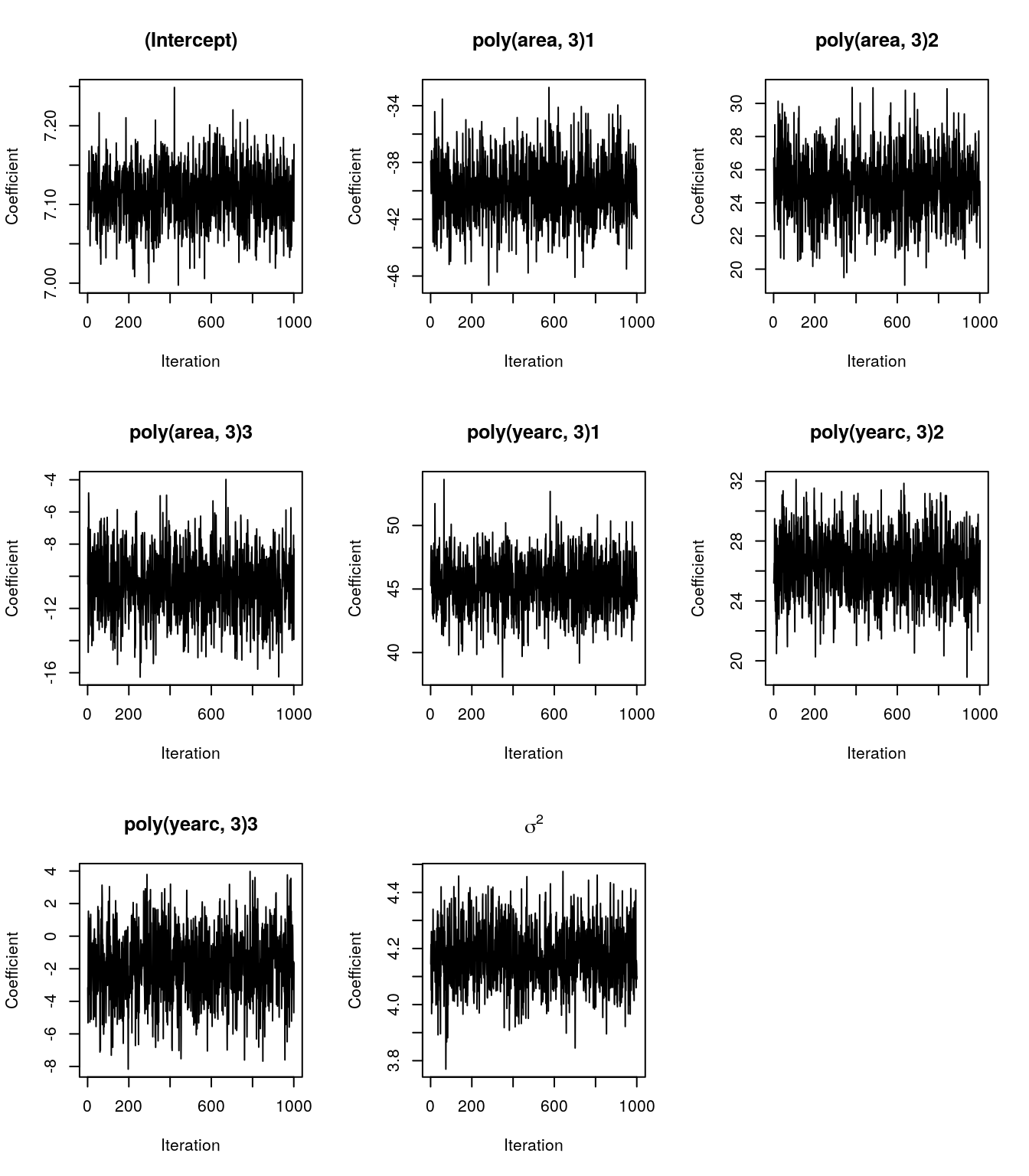

## Show summary output.
print(b)

## Call:
## gibbslm(formula = rentsqm ~ poly(area, 3) + poly(yearc, 3), data = MunichRent)
## ---
## Estimated coefficients:
##                   Mean   Sd   2.5%    50%  97.5%
## (Intercept)       7.11 0.04   7.04   7.11   7.18
## poly(area, 3)1  -39.86 2.14 -43.94 -39.87 -35.64
## poly(area, 3)2   25.03 1.95  21.16  25.03  28.97
## poly(area, 3)3  -10.52 1.97 -14.58 -10.53  -6.62
## poly(yearc, 3)1  45.39 2.08  41.30  45.44  49.16
## poly(yearc, 3)2  26.35 2.10  22.31  26.42  30.31
## poly(yearc, 3)3  -1.86 2.09  -6.21  -1.84   2.18
## ---
## Scale estimate
##        Mean   Sd 2.5%  50% 97.5%
## Sigma2 4.17 0.11 3.97 4.17  4.39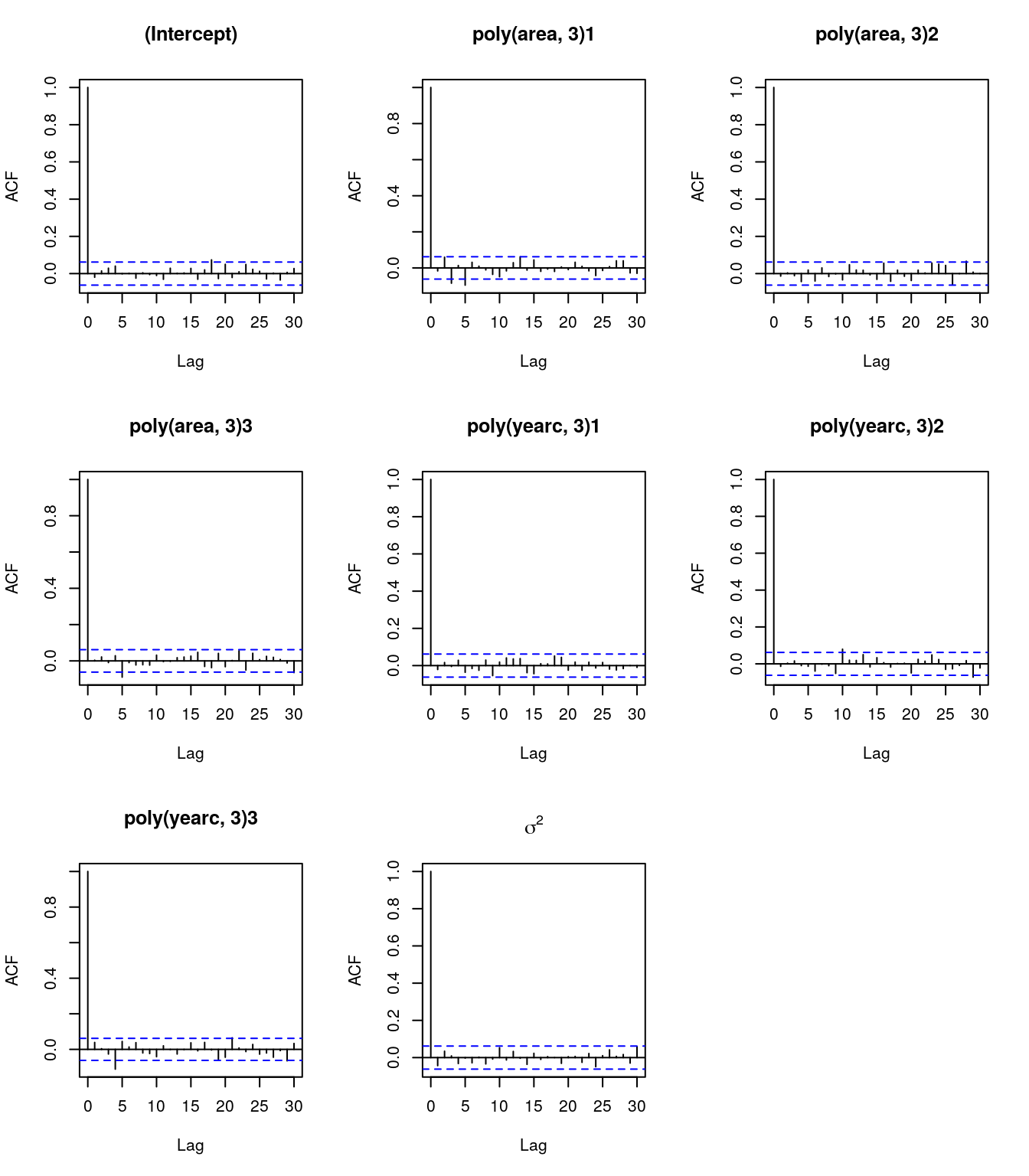

To visualize the effects we can write a small predict method.

## A simplified predict method, mainly copied from predict.lm().
predict.gibbslm <- function(object, newdata, FUN = c95) {
  ## Note, c95() is specified previously.
  ## All we need for prediction is the new design matrix.
  class(object) <- "lm"
  tt <- terms(object)
  if(missing(newdata) || is.null(newdata)) {
    X <- model.matrix(object)
  } else {
    Terms <- delete.response(tt)
    m <- model.frame(Terms, newdata, xlev = object$xlevels)
    if(!is.null(cl <- attr(Terms, "dataClasses"))) 
      .checkMFClasses(cl, m)
    X <- model.matrix(Terms, m, contrasts.arg = object$contrasts)
  }

  ## Compute predictions.
  p <- apply(object$samples$beta, 1, function(beta) { X %*% beta })


  ## Apply function on predicted values.
  p <- t(apply(p, 1, FUN))

  return(as.data.frame(p))
}

## Predict for each covariate, holding the other fixed
## at the mean. This way we can visualize the effects.
area <- seq(min(MunichRent$area), max(MunichRent$area), length = 100)
yearc <- seq(min(MunichRent$yearc), max(MunichRent$yearc), length = 100)

nd <- data.frame(
  "area" = area,
  "yearc" = mean(MunichRent$yearc)
)

p_area <- predict(b, newdata = nd)

## Same for variable yearc.
nd$yearc <- yearc
nd$area <- mean(MunichRent$area)

p_yearc <- predict(b, newdata = nd)

## Center effects to compare.
p_area <- p_area - mean(p_area$Mean)
p_yearc <- p_yearc - mean(p_yearc$Mean)
ylim <- range(c(p_area, p_yearc))

## Plot estimated effects.
par(mfrow = c(1, 2), mar = c(4.1, 4.1, 0.1, 1.1))
matplot(area, p_area, type = "l", lty = c(2, 1, 2), ylim = ylim, col = "black",
  xlab = "area", ylab = "Effect of area")
matplot(yearc, p_yearc, type = "l", lty = c(2, 1, 2), ylim = ylim, col = "black",
  xlab = "yearc", ylab = "Effect of yearc")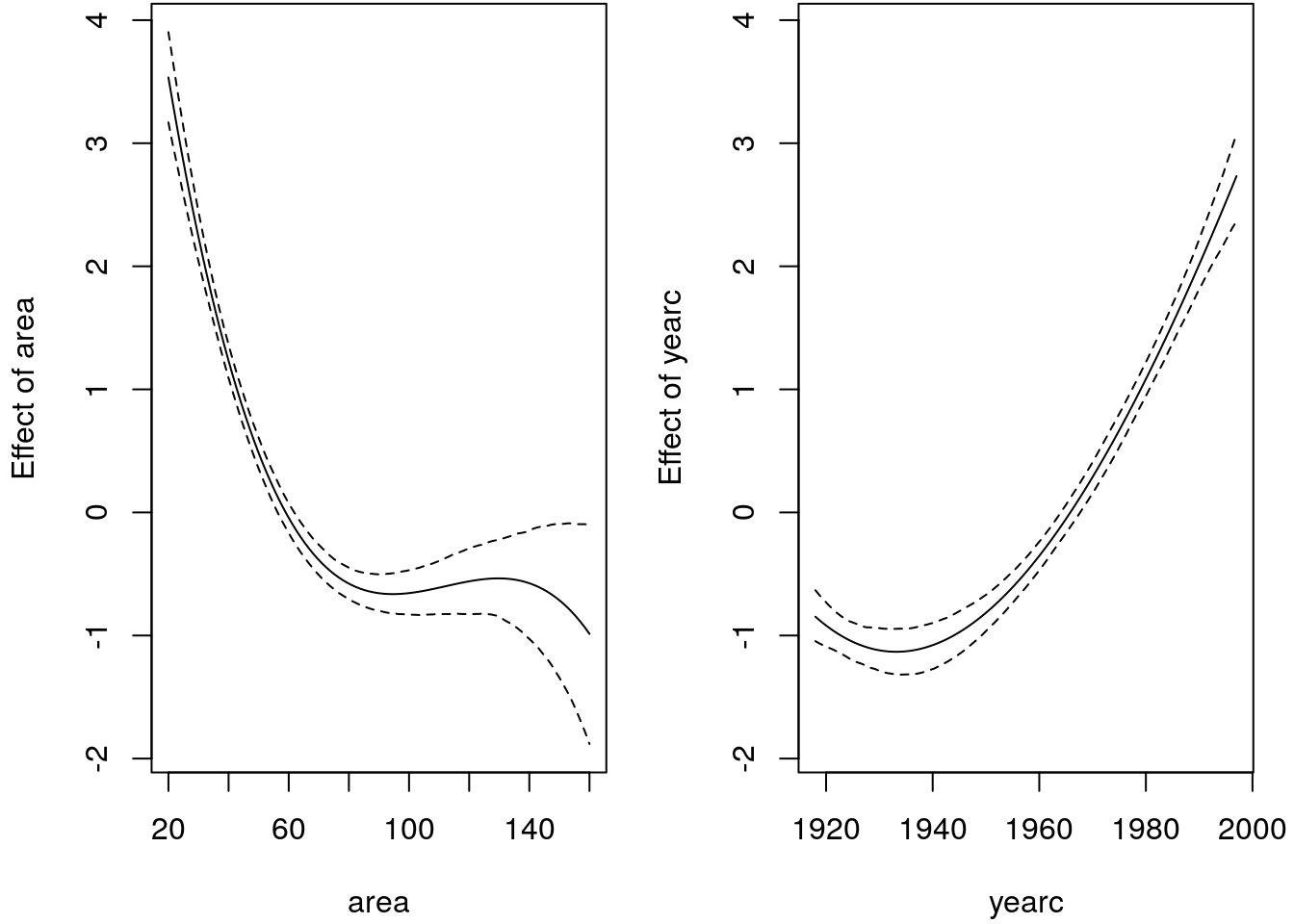

The estimated effects look really reasonable, in combination with the traceplots and the ACF plots, this implementation really seems to work and we can now estimate Bayesian linear models using Gibbs sampling. For sure, the implementation is not complete and could be improved, but this is up to you!

6.3 Bayesian P-splines

In section P-splines we discussed B-spline basis function with penalties, penalized splines can also be derived in a Bayesian framework. Moreover, the framework we present in this section is quite generic and works also for other types of smoothers. In particular, this allows us to employ Bayesian approaches for the estimation of P- splines including the smoothing parameter.

Lets start with the observation model \[ y_i = f(z_i) + \varepsilon_i = \sum_{j = 1}^k \gamma_jB_j(z_i) + \varepsilon_i \qquad \varepsilon_i \sim N(0, \sigma^2), \] with B-spline basis functions \(B_j\).

Instead of imposing a penalty, we will now develop an appropriate prior assumption for \(\boldsymbol{\gamma}\) that enforces a smooth function estimation.

Priors of regression coefficients

The stochastic analogue for the difference penalty are random walks of order \(k\) (RW\(k\)). A random walk of first order (RW\(1\)) is defined by \[ \gamma_j = \gamma_{j - 1} + u_j, \quad u_j \sim N(0, \tau^2), \quad j = 2, \ldots, d, \] or equivalently \[ \gamma_j - \gamma_{j - 1} = u_j, \quad u_j \sim N(0, \tau^2), \quad j = 2, \ldots, d, \] so that a connection to the first order difference penalty is recognizable.

We have to make further assumptions for the prior of the starting value \(\gamma_1\) and a non-informative prior distribution, \(p(\gamma_1) \propto const\) will be our standard option.

When considering the conditional distributions defined by a RW\(1\), we have \[ \gamma_j|\gamma_{j - 1}, \ldots, \gamma_1 \sim N(\gamma_{j - 1}, \tau^2). \] The RW\(1\) has a special dependence structure such that the conditional distribution of \(\gamma_j\) given all previous values is only dependent on the value lagged by one, i.e., \(\gamma_{j - 1}\). Therefore, the RW\(1\) has the (first order) Markov property. According to this formulation, the conditional expectation of \(\gamma_j\) is simply the lagged value \(\gamma_{j - 1}\) such that we obtain a constant trend for the expected value. This is illustrated in the following graphic.

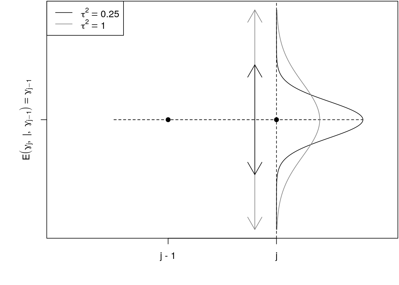
The deviations from parameter \(\gamma_{j-1}\) to \(\gamma_j\) are driven by the variance parameter \(\tau^2\), if \(\tau^2\) is small there is a strong penalty on neighboring coefficients, i.e., the larger \(\tau^2\) the more wiggly will be the smooth function. A constant value of all B-spline coefficients leads to a constant estimate for the function \(f(z)\). This corresponds to the case that the variance of the RW\(1\) is (almost) zero, since only very little deviation between \(\gamma_j\) and \(\gamma_{j - 1}\) is allowed in this situation resulting in a (near) constant trend for the sequence \(\gamma_1, \ldots, \gamma_d\). It follows that we can interpret the variance parameter \(\tau^2\) as related to an inverse smoothing parameter.

Joint (generic) prior

The joint multivariate prior distribution for \(\boldsymbol{\gamma}\) is then given by \[\begin{eqnarray*} p(\boldsymbol{\gamma} | \tau^2) &=& \prod_{j = 1}^k p(\gamma_j | \gamma_{j - 1}, \ldots, \gamma_1) \\ &=& p(\gamma_1) \prod_{j = 2}^k p(\gamma_j | \gamma_{j - 1}) \\ &\propto& \prod_{j = 2}^k \frac{1}{\sqrt{2\pi\tau^2}} \exp\left(-\frac{1}{2\tau^2}(\gamma_j - \gamma_{j - 1})^2\right) \\ &=& \frac{1}{(2\pi\tau^2)^{(k - 1)/2}} \exp\left(-\frac{1}{2\tau^2}\sum_{j = 2}^kd(\gamma_j - \gamma_{j-1})^2\right) \\ &=& \frac{1}{(2\pi\tau^2)^{(k - 1)/2}} \exp\left(-\frac{1}{2\tau^2}\boldsymbol{\gamma}^\top \mathbf{K}_1\boldsymbol{\gamma}\right). \end{eqnarray*}\] Combining the log-prior with the log-likelihood for posterior estimation we immediately see the connection to the frequentist approach, i.e., the log-posterior in the Bayesian setting is the penalized log-likelihood for the frequentist approach, see section Penalized regression.

Moreover, the multivariate normal prior can even be applied to other types of basis functions. A general smoothness prior is given by \[ p(\boldsymbol{\gamma} | \tau^2) \propto \left(\frac{1}{\tau^2}\right)^{rk(\mathbf{K}) / 2} \exp\left(-\frac{1}{2\tau^2}\boldsymbol{\gamma}^\top\mathbf{K}\boldsymbol{\gamma}\right). \]

6.4 Bayesian additive models

Using the general smoothness prior of the last section we can now specify full Bayesian Smooth additive models. The posterior of an additive model is then given by \[\begin{eqnarray*} p(\boldsymbol{\theta} | \mathbf{y}) &\propto& \frac{1}{(\sigma^2)^{\frac{n}{2}}} \exp\left( -\frac{1}{2 \sigma^2}\left(\mathbf{y} - \boldsymbol{\eta} \right)^\top \left(\mathbf{y} - \boldsymbol{\eta}\right)\right) \\ && \prod_{j = 1}^q \frac{1}{(\tau_j^2)^{rk(\mathbf{K}_j) / 2}} \exp\left(-\frac{1}{2\tau_j^2} \boldsymbol{\gamma}_j^\top\mathbf{K}_j\boldsymbol{\gamma}_j\right) \\ && \prod_{j = 1}^q (\tau_j^2)^{-a_j - 1} \exp\left(-\frac{b_j}{\tau_j^2} \right) \\ && (\sigma^2)^{- a_{\sigma^2} - 1} \exp \left(- \frac{b_{\sigma^2}}{\sigma^2} \right). \end{eqnarray*}\] Here, the priors for each smoothing variance \(\tau^2\) are most commonly inverse Gamma priors. Similar to the Bayesian normal linear regression model we derived in section Gibbs sampling, we obtain a multivariate normal full-conditional \[ \boldsymbol{\gamma}_j | \cdot \, \sim N(\mathbf{m}_j, \boldsymbol{\Sigma}_j) \] with expectation and covariance matrix \[\begin{eqnarray*} \mathbf{m}_{j} & = & E(\boldsymbol{\gamma}_j | \cdot) = \left(\frac{1}{\sigma^2}\mathbf{Z}_j^\top\mathbf{Z}_j + \frac{1}{\tau^2_j}\mathbf{K}_j \right)^{-1} \frac{1}{\sigma^2}\mathbf{Z}_j^\top(\mathbf{y} - \boldsymbol{\eta}_{-j}) \\ \boldsymbol{\Sigma}_j &=& Cov(\boldsymbol{\gamma}_j | \cdot) = \left(\frac{1}{\sigma^2}\mathbf{Z}_j^\top\mathbf{Z}_j + \frac{1}{\tau^2_j}\mathbf{K}_j \right)^{-1}. \end{eqnarray*}\] The full conditional of the parametric coefficients has expectation and covariance matrix \[\begin{eqnarray*} \mathbf{m}_{\boldsymbol{\beta}} &=& E(\boldsymbol{\beta} | \cdot) = \left(\mathbf{X}^\top\mathbf{X}\right)^{-1} \mathbf{X}^\top(\mathbf{y} - (\boldsymbol{\eta} - \mathbf{Z}_1\boldsymbol{\gamma}_1 - \ldots - \mathbf{Z}_q\boldsymbol{\gamma}_q)) \\ \boldsymbol{\Sigma}_{\boldsymbol{\beta}} &=& Cov(\boldsymbol{\beta} | \cdot) = \frac{1}{\sigma^2}(\mathbf{X}^\top\mathbf{X})^{-1}. \end{eqnarray*}\] For the variance parameters, we obtain \[\begin{eqnarray*} \tau^2_j | \cdot &\sim& IG(a_j + 0.5 rk(\mathbf{K}_j), b_j + 0.5 \boldsymbol{\gamma}_j^\top \mathbf{K}_j \boldsymbol{\gamma}_j), \\ \sigma^2 | \cdot &\sim& IG(a_{\sigma^2} + 0.5n, b_{\sigma^2} + 0.5(\mathbf{y} - \boldsymbol{\eta})^\top(\mathbf{y} - \boldsymbol{\eta})). \end{eqnarray*}\]

6.5 The R package bamlss

Bayesian Smooth additive models (and more, see the upcoming chapters) can be estimated using the R package bamlss. The main model fitting function is bamlss() and the most important arguments are:

bamlss(formula, family = "gaussian", data = NULL,
  weights = NULL, subset = NULL, offset = NULL,
  na.action = na.omit, ...)

The setup is in principal the same as the main model fitting function gam() of the mgcv package, i.e., all smooth terms that are part of mgcv can also be used in bamlss, see also section R package mgcv.

In the same way, a nonlinear smooth function of a covariate z can be modelled by

b <- bamlss(y ~ s(z), data = d)

We again exemplify the setup using the Munich rent index data MunichRent and estimate a Bayesian additive model of the form \[ \texttt{rentsqm}_i = \beta_0 + f(\texttt{area}_i) + f(\texttt{yearc}_i) + \varepsilon_i. \] The model is estimated in R with

## Load the library.
library("bamlss")

## Load the data.
load("data/MunichRent.rda")

## Model formula.
f <- rentsqm ~ s(area) + s(yearc)

## Set the seed.
set.seed(123)

## Estimate model.
b <- bamlss(f, data = MunichRent, n.iter = 12000, burnin = 2000, thin = 10)

Note that bamlss() first initializes regression coefficients and smoothing variances using posterior mode estimation with a Backfitting algorithm. Afterwards a full MCMC sampler is started with the estimated parameters from the backfitting step as starting values. Here, we specified the number of iterations (n.iter), the burn-in phase (burnin) and the thining parameter (thin). The defaults are a bit less, i.e., n.iter = 1200, burnin = 200 and thin = 1, this way the user can get a quick first estimate and does not need to wait too long if the model is more complex.

Similar to the mgcv package, we can plot the centered estimated effects with

par(mfrow = c(1, 2), mar = c(4.1, 4.1, 0.1, 1.1))
plot(b)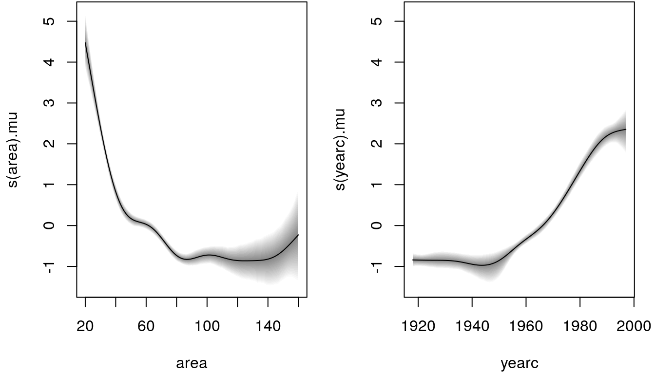

A summary method for the returned fitted model object exists

summary(b)

## 
## Call:
## bamlss(formula = f, data = MunichRent, n.iter = 12000, burnin = 2000, 
##     thin = 10)
## ---
## Family: gaussian 
## Link function: mu = identity, sigma = log
## *---
## Formula mu:
## ---
## rentsqm ~ s(area) + s(yearc)
## -
## Parametric coefficients:
##              Mean  2.5%   50% 97.5% parameters
## (Intercept) 7.112 7.039 7.112 7.178      7.111
## -
## Acceptance probability:
##       Mean 2.5% 50% 97.5%
## alpha    1    1   1     1
## -
## Smooth terms:
##                   Mean    2.5%     50%   97.5% parameters
## s(area).tau21   53.000  13.362  39.507 171.183     36.051
## s(area).alpha    1.000   1.000   1.000   1.000         NA
## s(area).edf      7.202   6.044   7.226   8.280      7.091
## s(yearc).tau21  10.408   0.804   5.598  45.121    143.622
## s(yearc).alpha   1.000   1.000   1.000   1.000         NA
## s(yearc).edf     5.558   3.714   5.522   7.727      8.381
## ---
## Formula sigma:
## ---
## sigma ~ 1
## -
## Parametric coefficients:
##               Mean   2.5%    50%  97.5% parameters
## (Intercept) 0.7065 0.6806 0.7058 0.7323      0.703
## -
## Acceptance probability:
##         Mean   2.5%    50% 97.5%
## alpha 0.9925 0.9409 1.0000     1
## ---
## Sampler summary:
## -
## DIC = 13118.92 logLik = -6551.553 pd = 15.816
## runtime = 56.631
## ---
## Optimizer summary:
## -
## AICc = 13114.1 edf = 17.4723 logLik = -6539.475
## logPost = -6620.66 nobs = 3082 runtime = 0.183

indicating high acceptance rates as reported by the alpha parameters in the model output, which is a sign of good mixing of the MCMC chains. The mixing can also be inspected graphically by

plot(b, which = "samples")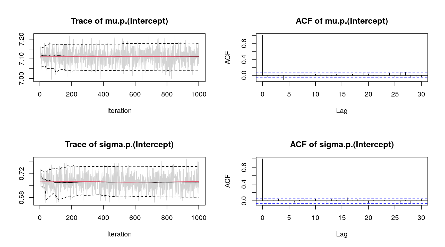

Note, for convenience we only show the traceplots of two parameters.

There are a couple more extractor functions implemented, like predict(), residuals(), samples(), etc. For a detailed introduction visit the project website http://bamlss.org/.

References

Hastings, W. K. 1970. “Monte Carlo Sampling Methods Using Markov Chains and Their Applications.” Biometrika 57 (1): 97–109. https://doi.org/10.1093/biomet/57.1.97.

Neal, Radford M. 2003. “Slice Sampling.” The Annals of Statistics 31 (3): 705–67. https://doi.org/10.1214/aos/1056562461.