Radiation Transport with Julia

The radiation transport equation

In this workshop, we wish to use a programming example from radiation transport. Do not worry, if you do not understand all details. Essentially everything boils down to solving a simple matrix ordinary differential equation. And if that sounds complicated, we can also say it boils down to matrix vector multiplications that your code should execute in the end.

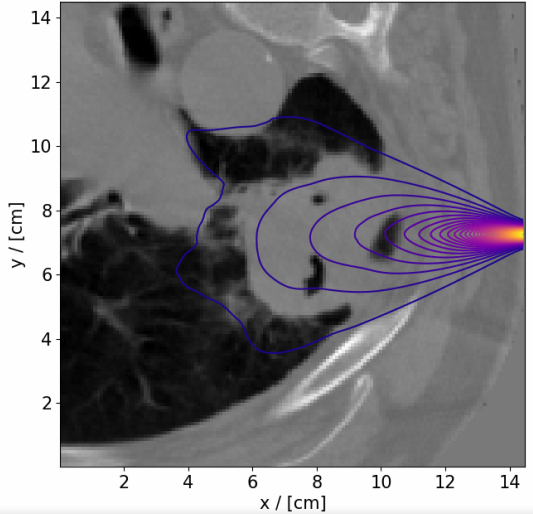
So let us give a little bit of background: The radiation transport equation describes radiation particles moving through a background material. In a one-dimensional geometry, particles can travel into directions $v\in [-1, 1]$ and are located at a spatial position $x\in[0, 1]$. One application which requires the simulation of radiation particles is radiation therapy, where photons are shot at a tumor to destroy cancerous cells. The radiation received by the patient is stored in a matrix $\bm{\psi}\in\mathbb R^{n_x \times n_{v}}$, where $n_x$ is the number of spatial cells and $n_v$ is the number of velocities. Below you find an example of a treatment planning result from radiation oncology. The treatment is chosen to destroy the lung tumor without harming important organs.

Adding packages

Let us first generate the velocity grid, which are commonly chosen to be the so-called Gauss-Legendre points. Luckily, these points are already implemented in Julia. All we need to do is to install the Julia Package FastGaussQuadrature. The $\operatorname{nv} = 10$ points can be accessed and stored in a vector $v$ by calling v, w = gausslegendre(nv). Note that $v$ contains the Gauss-Legendre points and $w$ contains the so-called quadrature weights used to compute integrals. Recall that it can be advantageous to create a new environment for this project.

shell> mkdir LinearTransportSolver

shell> cd LinearTransportSolver
/home/jonas/Projects/LinearTransportSolver

(SummerSchool) pkg> activate .
  Activating new project at `~/Projects/LinearTransportSolver`

(LinearTransportSolver) pkg> add FastGaussQuadrature

using FastGaussQuadrature
nv = 10
v, w = gausslegendre(nv)

Array generation and access

Now, to generate the spatial positions on which we want to evaluate the solution we can use the range command. Build a spatial grid $x\in\mathbb{R}^{n_x}$, with $n_x = 101$, where $x$ contains the spatial positions from $x_0 = 0$ to $x_1 = 1$.

nx = 101
x = collect(range(0, 1; length=nx))

The next step is to set up our solution matrix $\bm{\psi}$. The matrix should have dimension $\operatorname{nx}\times\operatorname{nv}$. Initially, the solution is zero except for $\psi_{50,k}=1$ for all $k$. Compute the described matrix.

ψ = zeros(nx, nv)

ψ[50, :] = ones(nv)

Linear algebra operations

A next step would be to evolve these particles in time. This is done by solving an ordinary differential equation of the form

Here $\mathbf{D}^{\pm}$ are tridiagonal matrices of the form

and

where $\Delta x = \frac{1}{n_x - 1}$. Set up these two matrices in your code.

(LinearTransportSolver) pkg> add LinearAlgebra

using LinearAlgebra
Δx = 1 / (nx - 1)
DPlus = (1 / Δx) * Tridiagonal(-ones(nx - 1), ones(nx), zeros(nx - 1))
DMinus = (1 / Δx) * Tridiagonal(zeros(nx - 1), -ones(nx), ones(nx - 1))

The matrices $\mathbf{V}^{\pm}\in\mathbb{R}^{n_v\times n_v}$ are diagonal matrices, where $\mathbf{V}^-$ collects all negative velocities on the diagonal, i.e., $\mathbf{V}^- = \text{diag}(v_1,\cdots,v_{5},0,\cdots,0)$ and $\mathbf{V}^+$ collects all positive velocities, i.e., $\mathbf{V}^+ = \text{diag}(0,\cdots,0,v_{6},\cdots,v_{10})$. Implement these two matrices. To write your code for general $\operatorname{nv}$, use the ceil and floor commands.

midMinus = Int(ceil(nv / 2))
midPlus = Int(floor(nv / 2))
VMinus = Diagonal([v[1:midMinus]; zeros(midPlus)])
VPlus = Diagonal([zeros(midMinus); v[(midPlus + 1):end]])

Lastly, the so called scattering matrix $\mathbf{G}$ is given as

Implement this matrix. You can try to not use for loops to test your element-wise operation skills.

G = ones(nv, nv) .* w - I

Now, to update your solution $\bm\psi$ from $t=0$ to $t = \Delta t$, we approximate the time derivative by $\bm{\dot \psi} \approx (\bm\psi_{\mathrm{new}}-\bm\psi)/\Delta t$. Hence, we then get

Implement the above formular using a time step size $\Delta t = 0.01$. Try to use dot operations whenever possible. You can already check how the solution has changed by inspecting ψ_new in the center. You already know how this works. If you want you can interpret the physical process that you observe.

Δt = 0.01;
ψ_new = ψ .+ Δt .* (-DPlus * ψ * VPlus .- DMinus * ψ * VMinus .+ ψ * G)

julia> midIndex = Int(floor(nx / 2));

julia> ψ_new[(midIndex - 1):(midIndex + 1), :]

Loops

Now, we do not want to know the solution at $\Delta t$, but at $t_{\mathrm{end}}=1.0$. If we just choose $\Delta t=1.0$ our approximation of the time derivative is inaccurate. Therefore, we wish to repeat the update with $\Delta t = 0.01$ fourty times. Use a loop to implement the repeated updates

nT = 40
ψ_new = zeros(size(ψ));

for n in 1:nT
    ψ_new .= ψ .+ Δt .* (-DPlus * ψ * VPlus .- DMinus * ψ * VMinus .+ ψ * G)
    ψ .= ψ_new
end

Now, we are interested in plotting $\phi(t_{\mathrm{end}},x) := \int_{-1}^1 \psi(t_{\mathrm{end}},x,v)\, \mathrm{d}v$. On a numerical level, we can compute this via

Φ = zeros(nx)

for j in 1:nx
    Φ[j] = sum(ψ[j, :] .* w)
end

Plotting

Luckily, Julia can include the Plots package. Install and add it to your code. Then run

using LaTeXStrings
using Plots; gr()

plot(x, Φ, labels=L"\Phi")
xlabel!("x")

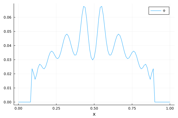
The output that you should get is

What you see is the particle density $\Phi$ over the spatial domain. Congratulations, you have just computed your first radiation transport problem using Julia. If you look at your code, you will see that it looks quite messy. you can add a comment test comment with # test comment. Use the comment command to explain what you did and double check if you understood everything. Also, commonly the using commands are executed in the first lines of the code, so move all these commands to the top.

Element-wise operations

To better understand element-wise operations, see how we computed the scattering matrix $\mathbf{G}$ and see if you can write this in terms of for-loops. You can use the if command.

G = zeros(nv, nv);

for i in 1:nv
    for j in 1:nv
        G[i, j] = w[i]
        if i == j
            G[i, j] = G[i, j] - 1
        end
    end
end

Full sample solution

using FastGaussQuadrature
using LaTeXStrings
using LinearAlgebra
using Plots; gr()

# define velocity grid according to gauss quadrature
nv = 10
v, w = gausslegendre(nv)
nx = 101
x = collect(range(0, 1; length=nx))

# setup initial condition
ψ = zeros(nx, nv)
ψ[50, :] = ones(nv)

# create stencil matrices
dx = 1 / (nx - 1)
DPlus = (1 / dx) * Tridiagonal(-ones(nx - 1), ones(nx), zeros(nx - 1))
DMinus = (1 / dx) * Tridiagonal(zeros(nx - 1), -ones(nx), ones(nx - 1))

# create system matrices
midMinus = Int(ceil(nv / 2))
midPlus = Int(floor(nv / 2))
VMinus = Diagonal([v[1:midMinus]; zeros(midPlus)])
VPlus = Diagonal([zeros(midMinus); v[(midPlus + 1):end]])

# create scattering matrix
G = ones(nv, nv) .* w - I

# allocate memory
ψ_new = zeros(size(ψ))

# advance in time
Δt = 0.01
nT = 40

for n in 1:nT
    ψ_new .= ψ .+ Δt .* (-DPlus * ψ * VPlus .- DMinus * ψ * VMinus + ψ * G)
    ψ .= ψ_new
end

# store phi for plotting
Φ = zeros(nx)

for j in 1:nx
    Φ[j] = sum(ψ[j, :] .* w)
end

# plot phi
plot(x, Φ, labels=L"\Phi")
xlabel!("x")