Supervised learning

The goal of supervised learning is to learn a function that maps inputs to outputs based on input data that has been labeled for a particular output. Usually, the algorithms fall into two categories:

• Classification tasks: Here, supervised learning tries to predict the category a data point belongs to. This is e.g. used in spam detection, speech recognition, describing images, or handwriting recognition.

• Regression tasks: Here, supervised learning is used to predict a continuous numerical value based on an input data point. This is e.g. used in sales forecasting or temperature forecasting.

In this section we will just look into one classification task and we will do so by applying K nearest neighbors (KNN).

We continue to work with the MNIST data set and since we are experimenting with supervised learning, we need to use the training as well as the test data set - including the labels.

In case we do not have X_train, X_test, y_train and y_test at hand, we can have a look at the following code:

using MLDatasets

df_train = MNIST(:train)
df_test = MNIST(:test)

X_train = reshape(df_train.features, (28 * 28, :))'
y_train = df_train.targets
X_test = reshape(df_test.features, (28 * 28, :))'
y_test = df_test.targets

Classification (K Nearest Neighbors)

Theory

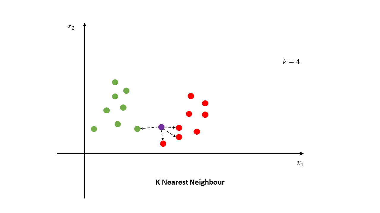
The K nearest neighbors is one of the simplest algorithms used for classification tasks. Recall that our data is $784$-dimensional and every data point corresponds to one handwritten digit. If we want to make a prediction for a previously unseen handwritten digit, we simply flatten the matrix, put the point in our $784$-dimensional space and find the $K$ nearest neighbors (depending on a predefined metric) within the training data set. We then look at the labels of these nearest neighbors and get a majority vote. So if most of the neighbors are of category $c$, then the prediction of the previously unseen handwritten digit would also be $c$. This image illustrates this process:

Application

Again we will use MLJ.jl to apply the KNN algorithm. The workflow stays exactly the same and we even have multiple implementations to choose from. In this workshop we will use the KNNClassifier from the NearestNeighborModels.jl package. Since we are already used to work with MLJ.jl, we will leave this as an exercise.

using DataFrames, MLJ, NearestNeighborModels

KNN = @load KNNClassifier pkg=NearestNeighborModels
model_knn = KNN(K=10)

X_train_tab = MLJ.table(X_train)
X_test_tab = MLJ.table(X_test)

y_train_cat = categorical(y_train)
y_test_cat = categorical(y_test)

mach_knn = machine(model_knn, X_train_tab, y_train_cat)
fit!(mach_knn)

pred_test = MLJ.predict(mach_knn, X_test_tab)
pred_vector = Vector{Int64}(mode.(pred_test))

Note that running predict is quite slow in this case. For every data point in the test set we need to find the $10$ nearest neighbors within the training data set. Thus, we need to compute $10000 * 60000$ matrices, which takes a while. After finishing the exercise, we should have a vector with predicted labels of previously unseen data (test set). Now we are interested in the quality of these predictions, so we compare them to real labels. One method to do so is the confusion matrix. Each column represents instances of the real (expected) value while each row represents the predicted value. The diagonal shows the correct predictions and every other matrix element the missclassifications. We will use the confusion matrix implementation that is available in the KnetMetrics.jl package since it supports confusion matrices with more than two classes.

julia> using KnetMetrics

julia> conf_mat = KnetMetrics.confusion_matrix(pred_vector, y_test)
conf_mat =

                                  Expected

      0      1      2      3      4      5      6      7      8      9
______________________________________________________________________
    972      0     13      0      2      4      6      0      6      7   │0 
      1   1132     12      3     11      0      4     27      4      6   │1 
      1      2    982      3      0      0      0      4      5      3   │2 
      0      0      2    976      0     12      0      0     11      7   │3 
      0      0      1      1    940      1      3      2      7     10   │4 
      2      0      0     10      0    863      2      0      9      3   │5	Predicted
      3      1      2      1      4      6    943      0      4      1   │6 
      1      0     17      7      1      1      0    983      7     10   │7 
      0      0      3      6      1      1      0      0    914      2   │8 
      0      0      0      3     23      4      0     12      7    960   │9

The confusion matrix tells us that our model is almost perfectly recognizing 0, 1, and 6, but is doing worse with classifying 2, 4, or 7 correctly. To get the accuracy, we can use the MLJ.accuracy function:

julia> MLJ.accuracy(pred_vector, y_test)
0.9665

So our KNN reached an accuracy of 96.7%, which is really amazing already. In case you are interested how other algorithms perform, have a look at the MNIST database article on Wikipedia.

Pluto Notebook